Central Moments

Overview

In the previous chapter, we explored the statistical concepts of a sample and populations as a starting point to explore frequency distributions, the Central Limit Theorem and some basic statistical tests. Many of these are based on key metrics like the mean, standard deviation, and the variance. But what are these metrics, exactly?

In this chapter, we focus on mean, variance and other summary statistics, which are based on the Frequency distribution of a trait. For our purposes, a trait is a set of measurements or observations that can be coded as a numeric vector in R. Typically, the observations might be a column in a data.frame or tibble object, as covered in the R Crash Course for Biologists book.

As you know from the last chapter, we can generate a frequency distribution for a trait if we plot the scale of the numeric vector on the x-axis, from lowest to highest value. Then, we bin similar values together and plot the frequency of each observation on the y-axis.

Frequency distributions are invaluable for exploring variation in your data. In the next chapter, we’ll see how frequency distributions are essential for quality assessment and quality controls in linear models for statistical analysis.

Once we have a frequency histogram, there are several summary statistics that we can use to characterize the distributions, based on the Central Moments of the data. Rather than try to define these in words, it’s much easier to understand central moments through R graphics, R objectcs, and a little bit of basic math.

The M word

If you are reading this book, you might think that you are are helpless at math, just as I did when I was a biology student. If you are like me, then your instinct is to skip any equations you see in a textbook or presentation. In this book, I will show you how to use R code to help make sense of math equations. To do this, you will have to stop yourself whenever you see a math equation, and dissect it down to individual terms. Each term in an equation can be coded as an object in R, and writing your own R code to put those objects together. Once you are comfortable coding simple equations in R, you will will quickly learn to program more complex equations by breaking them down into smaller code chunks. This will help you understand complex equations by forcing yourself to work through them slowly and in steps. I have deliberately kept this chapter short, so that you can spend more time working through the equations. Later, we will get into larger and more complex equations, so it’s important to spend the time now to develop your skills.

Setup

library(ggplot2) # plotting library

Warning: package 'ggplot2' was built under R version 4.5.2

source("http://bit.ly/theme_pub") # Set custom plotting theme
theme_set(theme_pub())

Central Moments

Central Moments (CM) are summary statistics that characterize the frequency distribution of a trait. If you are already comfortable with the calculation of the mean and variance, then you know all the math necessary to calculate central moments.

Let’s start with the mean:

\[\bar x = \frac{\sum(x_i)}{N}\]

Looks daunting, but it’s easy in R! the numerator is just the sum (\(\sum\)) of each measurement (\(x\)) across all individual elements of our vector (\(i\)). The numerator, is just the number of elements (\(N\)).

Let’s try this for a vector of 100 values drawn randomly from a normal distribution.

Try writing code for this in R.

Hint: Which function do we use to generate random numbers from a normal distribution? Which function will add together all the elements of a vector? How do we calculate the number of elements, and how do we divide them?

set.seed(123)
X<-rnorm(100)
(Mean<-sum(X)/length(X))

[1] 0.09040591

Once we have the mean, we can calculate the central moments. The second central moment is the variance:

\[\frac{\sum(x_i - \bar x)^2}{N-1}\]

The equation is not much different than the one above. Let’s break it down. The only real trick here is to be careful about how you use the brackets.

Brackets first. \(\bar x\) is just the mean, which we subtract from each value: x-mean(x). This is also called the deviation.
Next, we square each term. We use brackets to make sure we square the deviation, not just the mean: (x-mean(x))^2. If we exclude the extra brackets x-mean(x)^2, then our numerator would be \(\sum x_i -\bar x^2\), which means we would first sum all values of \(x\) before subtracting the square of the mean (\(\bar x^2\)) from it. Instead, we want to subtract each value from the mean and then square the difference.
Now add them together: sum((x-mean(x))^2). Note how we need the extra brackets inside of the sum() function, because we want to square each value of x, not the sum. If we did `sum(x-mean(x))^2, the numerator would be \([\sum (x_i - \bar x)]^2\).
Finally, we divide by the number of observations, minus one. Again, watch the brackets: sum((x-mean(x))^2)/(N-1) If we don’t have n-1 in brackets (sum((x-mean(x))^2)/N-1), R won’t follow the order of operations. Instead it will first divide the whole thing by \(N\) and subtract 1, which would be \(\frac{\sum(x_i - \bar x)^2}{N} -1\)

So the final equation is:

(Var<-sum((X-mean(X))^2)/(length(X)-1))

[1] 0.8332328

Once you understand the variance, the other central moments are very easy – just substitute the exponent:

The 2nd CM is the Variance: \(\frac{\sum(x_i - \bar x)^2}{N-1}\)
The 3rd CM is the Skewness: \(\frac{\sum(x_i - \bar x)^3}{N-1}\)
The 4th CM is the Kurtosis: \(\frac{\sum(x_i - \bar x)^4}{N-1}\)

Once you understand the equations, it’s easy to remember what the different moments are telling you about the frequency distribution. Let’s explore each one.

Variance

As explored in the previous chapter, the variance of a distribution is a measure of the spread of the data. The higher the variance, the more spread out the data are. You can see this in the equation: the numerator depends on the deviation (\(x_i - \bar x\)). So values far away from the mean are then squared, making the numerator bigger. This is why larger values of variance indicate data that are more spread out from the mean.

In biological data, the variance often scales with the mean, so it is often valuable to use the cofficient of variance (\(C_v\)), as discussed in the previous chapter.

Question Why is \(N-1\) in the denominator for the variance equation, rather than \(N\)?

Answer: This is a common source of confusion. Subtracting 1 from the variance reduces the denominator slightly, with more of an effect for small sample sizes. This is a deliberate adjustment to slightly inflate the variance estimates of small samples.

Coefficient of Skew

Notice that skew is like variance but with the third exponent, meaning that values can be negative or positive. If we have a few very small values (relative to the mean) then our skew will tend to be more negative. If we have a few very large values it will tend to be more positive. Skew will also increase with the variance of the distribution, so we often standardize using the standard deviation raised to the same exponent, which gives us the coefficient of skew:

\[ C_{Skew} = Skew/s^3 = \frac{\sum(x_i - \bar x)^3}{s^3(N-1)}\] A normal distribution will typically have a coefficient of skew near zero. Therefore

Negative \(C_{Skew}\) values usually indicate a distributions with left skew

Positive \(C_{Skew}\) values usually indicate a distributions with right skew

Values of \(C_{Skew}\) near zero are symmetical (i.e. ‘normal’)

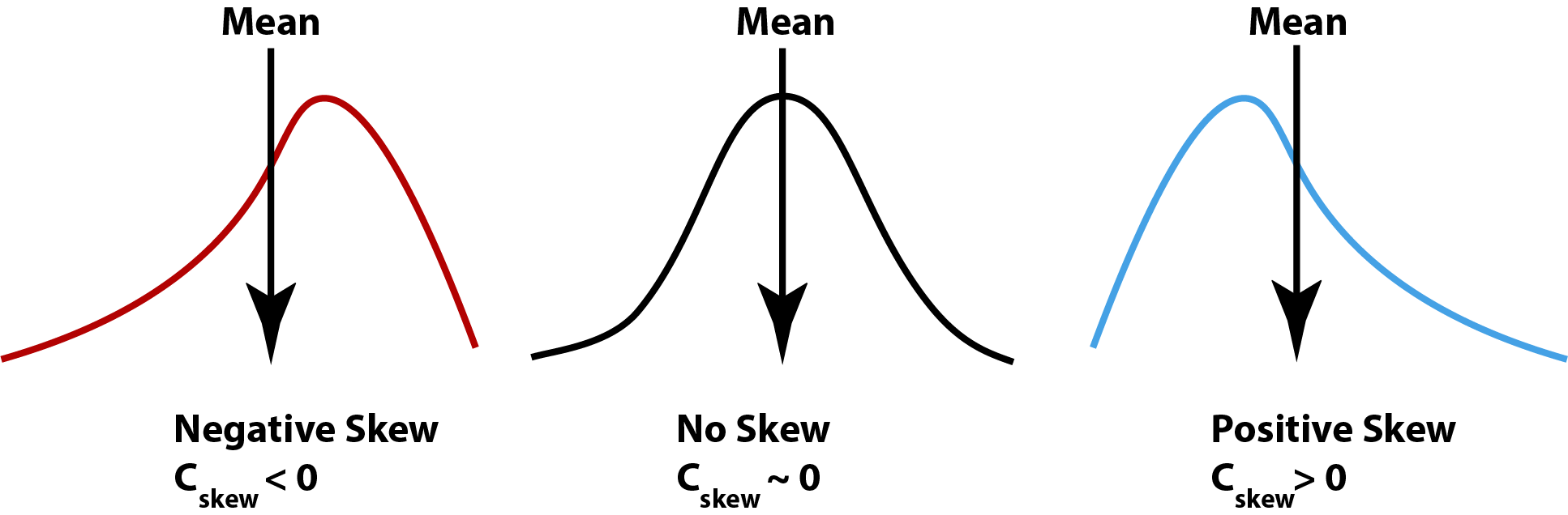
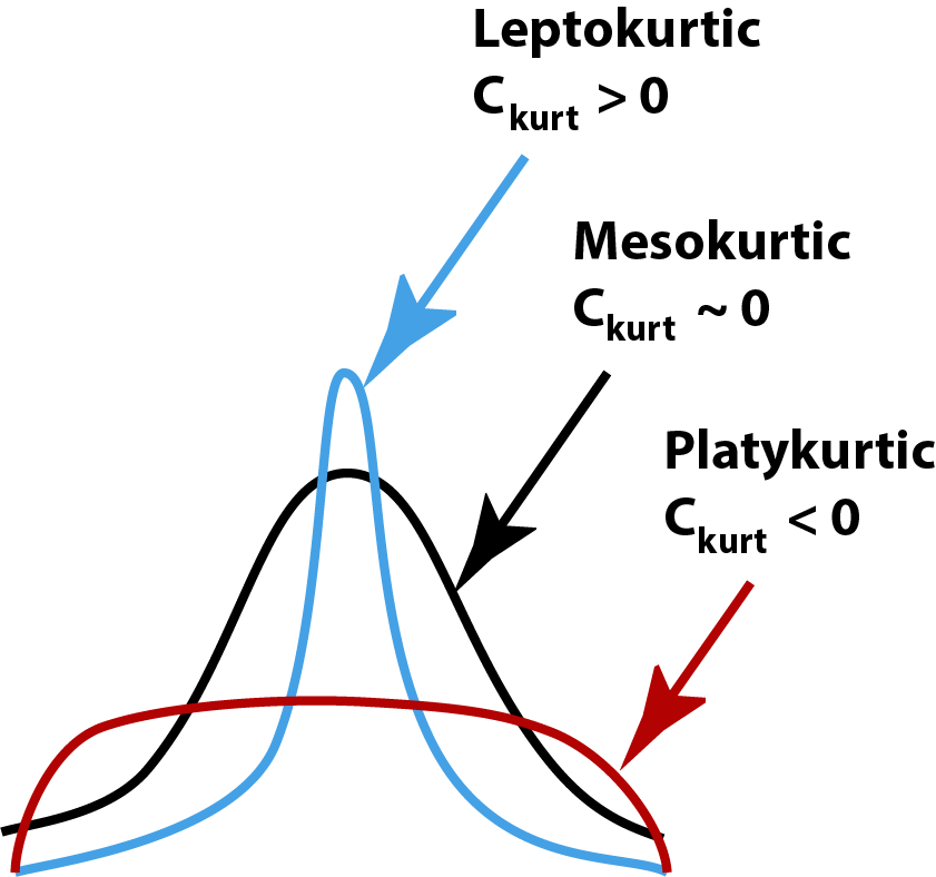
Coefficients of skew with corresponding mean and distribution examples

Coefficient of Kurtosis

Kurtosis uses the 4th exponent, so all values will be positive. By raising deviations to the 4th power, points farther from the mean are weighted more heavily than values close to the mean. Like Skew, kurtosis will also scale with the variance, so we usually calculate a coefficient of kurtosis, standardized in an analogous way, but this time we also subtract 3:

\[ C_{Kurt} = Kurt/s^4 = \frac{\sum(x_i - \bar x)^4}{s^4(N-1)} -3\] We subtract 3 because a normal distribution will typically have a coefficient of kurtosis near 3. This means that:

Positive \(C_{Kurt}\) values characterize Leptokurtic distributions, or ‘overdispersed’ data

Neative \(C_{Kurt}\) values characterize Platykurtic distributions, or ‘underdispersed’ data

Values of \(C_{Kurt}\) near zero are Mesokurtic distributions (i.e. ‘normal’)

Non-Normal Data

Now that we know how to use central moments to characterize non-normal distributions, let’s look at some examples. For each example, we will want to graph the frequency histogram and calculate the mean and central moments. Rather than write the same code for the central moments for each distribution,, we can write a custom function to output the mean, variance, and coefficients of skewness and kurtosis. We can make a custom function in R using the function() function. We set the input parameters in regular brackets () and the function itself in curly brackets {}.

Moments<-function(x=NA){
  Mout<-round(
    c(mean(x),
      var(x),
      sum((x-mean(x))^3)/(sd(x)^3*(length(x)-1)),
      sum((x-mean(x))^4)/(sd(x)^4*(length(x)-1)),
    digits=2))
  print(paste("Mean =",Mout[1]))
  print(paste("Var =",Mout[2]))
  print(paste("Cskew =",Mout[3]))
  print(paste("Ckurt =",Mout[4]))
}

The brackets for coefficients of skew and kurtosis are tricky here. Take a minute to look at each component carefully to understand why each bracket is needed where it is.

Let’s look at a few examples, starting with a normal distribution for comparison:

X<-NormDat<-rnorm(1000)
ggplot() + geom_histogram(aes(x=NormDat))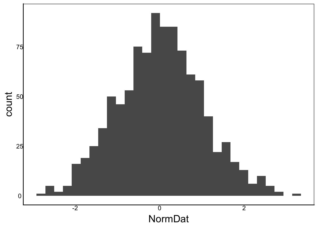

Moments(X)

[1] "Mean = 0"
[1] "Var = 1"
[1] "Cskew = 0"
[1] "Ckurt = 3"

What if we raise each value to the exponent: \(e^x\)

ExpDat<-exp(rnorm(1000))
ggplot() + geom_histogram(aes(x=ExpDat))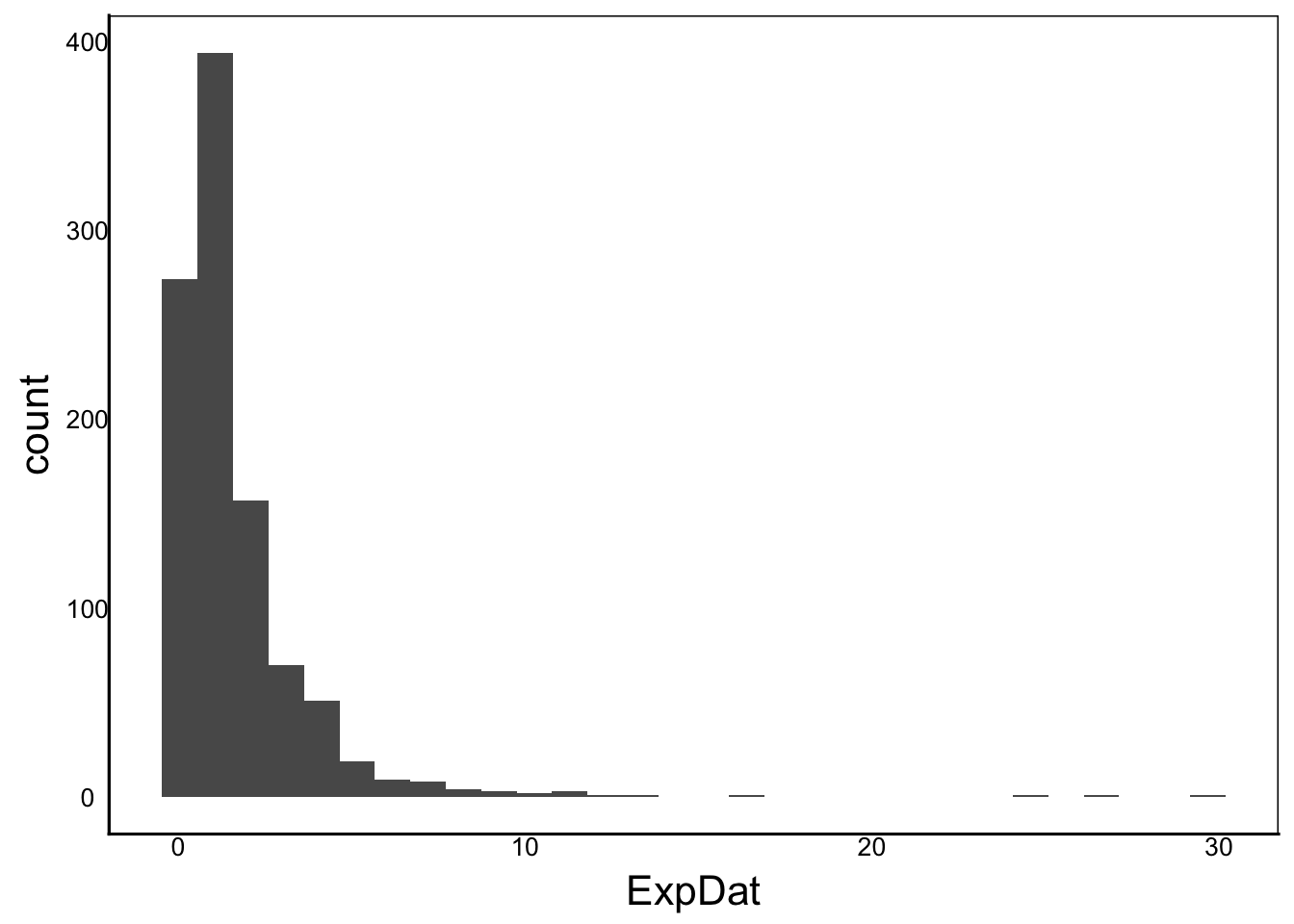

Moments(ExpDat)

[1] "Mean = 2"
[1] "Var = 5"
[1] "Cskew = 6"
[1] "Ckurt = 58"

Or multiply two randomly chosen values: \(x_i \times y_i\)

multNorm<-rnorm(1000)*rnorm(1000)
ggplot() + geom_histogram(aes(x=multNorm))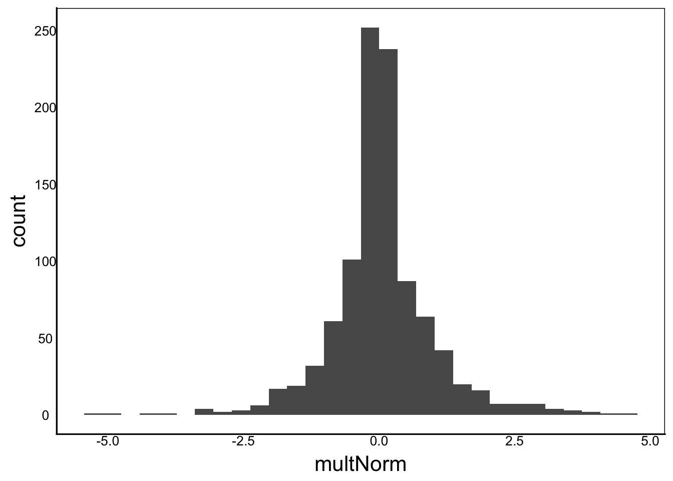

Moments(multNorm)

[1] "Mean = 0"
[1] "Var = 1"
[1] "Cskew = 0"
[1] "Ckurt = 8"

Or take the reciprocal: \(1/x_i\)

invNorm<-1/rnorm(1000)
ggplot() + geom_histogram(aes(x=invNorm))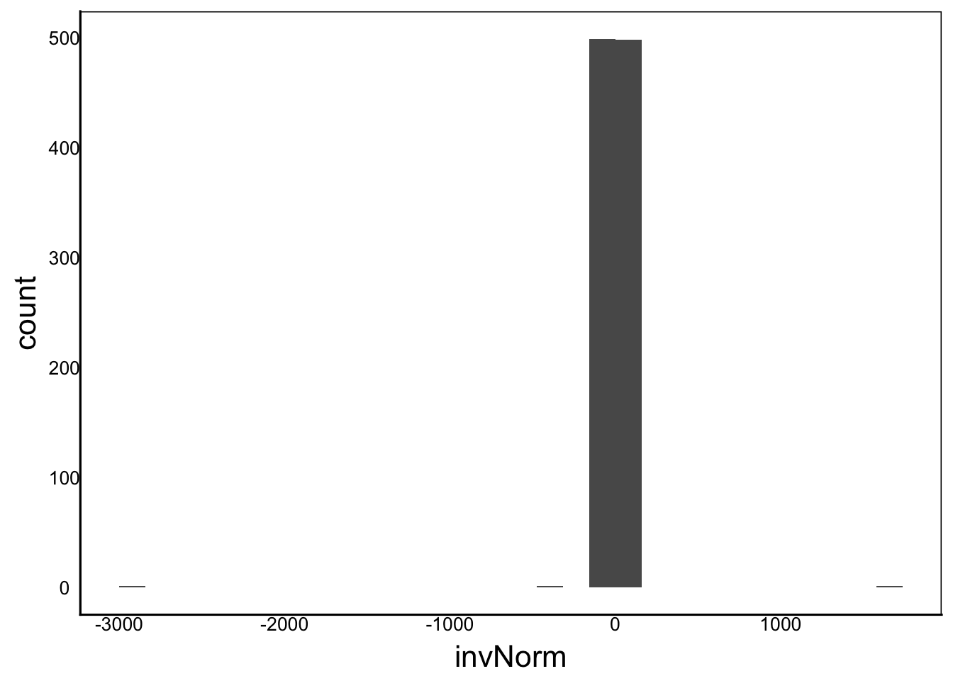

Moments(invNorm)

[1] "Mean = -1"
[1] "Var = 11476"
[1] "Cskew = -17"
[1] "Ckurt = 609"

Let’s try two more using different distributions that we know are not normal:

BinDat<-rbinom(n=1000, size=5, prob=0.2)
ggplot() + geom_histogram(aes(x=BinDat))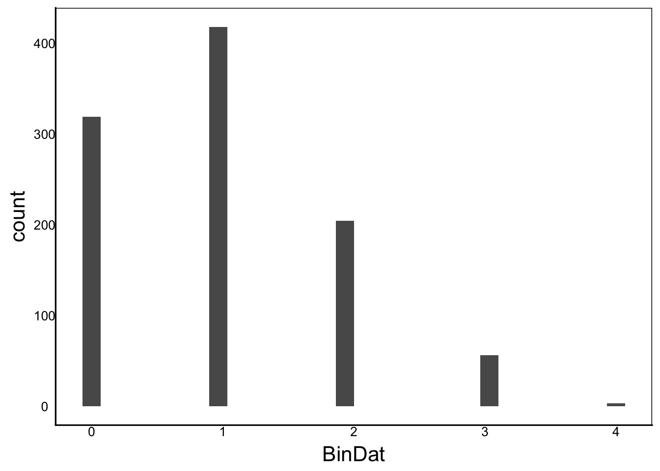

Moments(BinDat)

[1] "Mean = 1"
[1] "Var = 1"
[1] "Cskew = 1"
[1] "Ckurt = 3"

PoisDat<-rpois(n=1000, lambda=2)
ggplot() + geom_histogram(aes(x=PoisDat))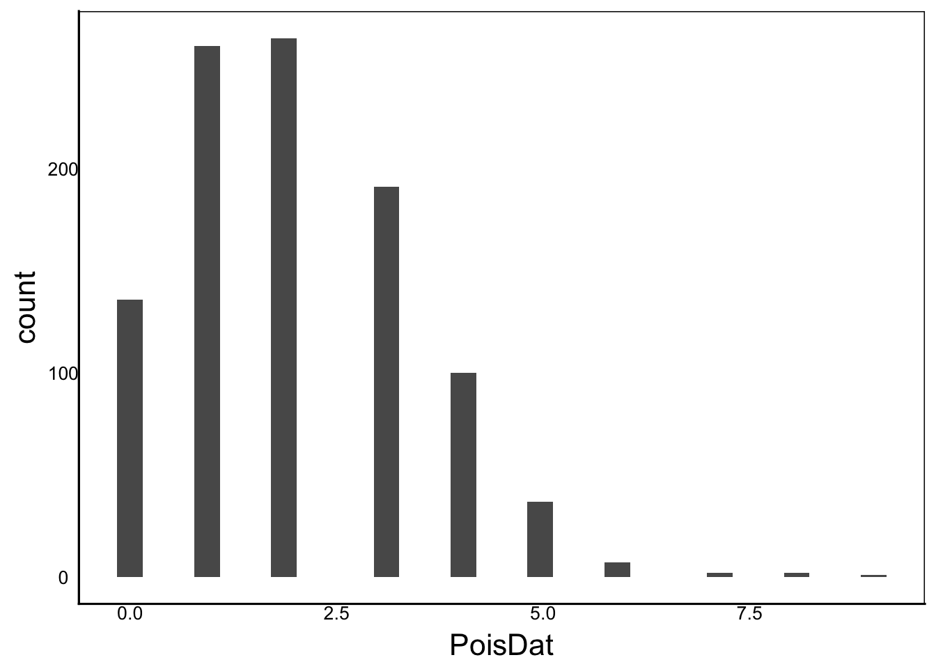

Moments(PoisDat)

[1] "Mean = 2"
[1] "Var = 2"
[1] "Cskew = 1"
[1] "Ckurt = 4"

Weigted Moments

Earlier, we saw that the variance is the second central moment, calculated by summing the squared deviations, weighted by the sample size.

\[\frac{\sum(x_i - \bar x)^2}{N-1}\]

However, this equation assumes each observation has equal weighting, with \(n\) equal to the number of observations. For example, what if we monitored the age of first reproduction of a long-lived seabird. To make the calculations easy, let’s assume we examine 100 randomly sampled individuals and obtain this table:

\(x_i\)	\(n_i\)	\(f_i\)
7	2	0.02
8	5	0.05
9	23	0.23
10	34	0.34
11	21	0.21
12	11	0.11
13	4	0.04
14	1	0.01

The table shows the Age of first reproduction (\(x_i\)), the number of birds observed at each age (\(n_i\)), and the fraction (\(f_i\)) of each category, which is just the number of observations of each row divided by the total (100).

Question: How can we calculate the variance for this table?

If we plot the data, they look like values we would get if we sampled a normal distribution:

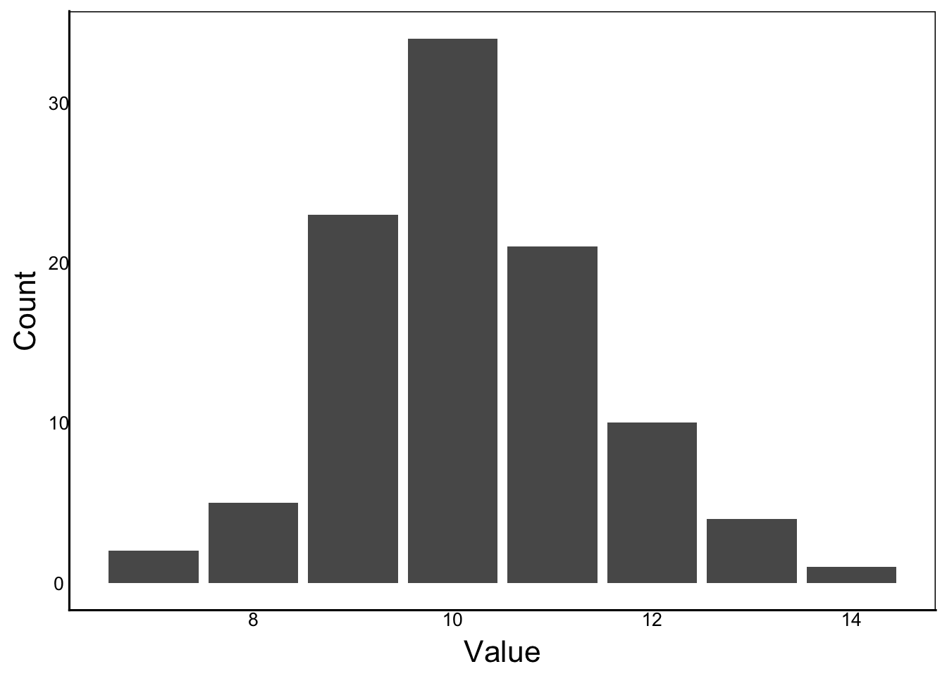
We could write code to repeat each Age the observed number of times: for example, enter 7 twice, 8 five times, etc. Alternatively, we can calculate a weighted variance. A weight is just a modifier that adjusts the value of observations, so a weighted variance adjusts each value by the proportion of observations. We can also calculated the weighted average in an analogous way:

\[\bar x = \frac{\sum n_ix_i}{N}\]

\[s^2 = \frac{\sum n_i(x_i - \bar x)^2}{N-1}\]

In these equations, the \(x_i\) is the value from the Age column, \(n_i\) is the number of birds observed at that age, and \(N\) is the total number of birds (100). In fact, we can simplify this even further, if we divide each \(n_i\) by the total, which give us the proportions as shown in the \(f_i\) column in the breeding bird table.

\[\bar x = \sum f_i x_i\]

We can apply the same formula to calculate the other central moment coefficients:

Variance: \(s^2 = \sum f_i(x_i - \bar x)^2\)
Coefficient of Skew: \(C_{skew} = \frac{\sum f_i(x_i - \bar x)^3}{s^3}\)
Coefficient of Kurtosis: \(C_{kurt} = \frac{\sum f_i(x_i - \bar x)^4}{s^4}\)

Technically, our variance has a slight bias because it translates to \(N\) instead of \(N-1\) in the denominator, but it’s a reasonable approximation for most modern biological data.

Expectations

Now imagine that we didn’t just sample 100 individuals, but we want to know the mean and variance for the entire population of seabirds, or an imaginary infinite population from which we could draw a sample. How would we do this? We could use the same approach: weight each observation by its proportion in the full population. Conventionally, these are written as expectations rather than weighted values, but they are conceptually the same.

The expectation of \(x\) is the mean:

\[E(x) = \sum f_i x_i\]

The first central moment is the average deviation:

\[E[x-E(x)] = \sum f_i (x_i-\bar x)\]

The second central moment, is the variance:

\[E[(x-E(x))^2] = \sum f_i (x_i-\bar x)^2\]

Similarly, we can calculate any central moment \(n\):

\[E[(x-E(x))^n] = \sum f_i (x_i-\bar x)^n\]

Covariance

Until now, we have considered only a single variable. What if we had a hypothesis that seabirds with brighter plumage were more developed and therefore more likely to breed earlier? We would expect brighter plumage colours for earlier years of reproduction in our earlier table. We can quantify this by modifying our second central moment. To start, consider that we can re-arrange the equation:

\[E[(x-E(x))^2] = E[(x-E(x))(x-E(x))]\]

This is really just multiplying the first central moment by itself. What if we replace one variable with our second variable? This is called the covariance.

\[COV = E[(x-E(x))(y-E(y))] = \sum f_i (x_i-\bar x)(y_i-\bar y)\]

So, if \(x_i\) is a younger age, we predict lighter plumage (i.e., higher \(y_i\)). Likewise, if \(x_i\) is an older age, we predict darker plumage values of \(y_i\).

Scaling

One problem with covariance and central moments is that they are scale-dependent. This makes them difficult to compare across studies or even across measurements of the same study. For example, imagine if we measure heights in meters and centimeters and try to compare the mean and variance:

Ht_m<-c(1.42,1.47,1.53,1.65,1.72)
Ht_cm<-Ht_m*100
var(Ht_m)

[1] 0.01557

var(Ht_cm)

[1] 155.7

Note the variance of the same trait is 10,000 times higher when measured in centimeters than in meters. There is no difference in the biology of these measurements, so it would be helpful to standardize them somehow.

One way to standardize, is to set the mean to zero and standard deviation to one, as we saw with z-scores in the Populations and Distributions Chapter. Standardizing each trait to z-scores makes covariances comparible, with values ranging from 1 for a strong positive association (higher \(x\) predicts higher \(y\)) to -1 for a strong negative association (higher \(x\) predicts lower \(y\)) through 0 for no association (\(x\) doesn’t predict \(y\)).

In addition to calculating covariance of z-scores, there are two other useful scaling methods that are commonly used in the analysis of biological data.

Correlation

Parametric

The Product-Moment correlation, sometimes called Pearson’s Correlation Coefficient scales the covariance by pooling variance of each trait:

\[r = \frac{COV_{x,y}}{\sqrt{V_x-V_y}} = \frac{\sum f_i (x_i-\bar x)(y_i-\bar y)}{\sqrt{\sum f_i (x_i-\bar x)^2 \sum f_i (y_i-\bar y)^2}}\]

Again, don’t be intimidated by the large equation. You already understand it, you just have to break it into pieces and fill in the values.

We can code it out together to help it stick:

\(x_i\) is a vector of numbers:

x<-c(-2,-1,0,1,2)

\(y_i\) is also a vector of numbers, which may be associated with x. In this case, let’s make a negative association by simply reversing the values of x:

y<-c(2,1,0,-1,-2)

We can also define a vector of weights (i.e., fractions). Since each value occurs once out of five elements in each vector, they all have the same weight of \(1/4\). Remember, we use \(N-1\) in the denominator for small sample size, which is why it is \(1/4\) instead of \(1/5\).

f<-rep(1/4,5)

The variance of x and y:

sum(f*(x-mean(x))^2)

[1] 2.5

var(x)

[1] 2.5

sum(f*(x-mean(y))^2)

[1] 2.5

var(y)

[1] 2.5

The covariance of x and y:

sum(f*(x-mean(x))*(y-mean(y)))

[1] -2.5

cov(x,y)

[1] -2.5

And finally the correlation of x and y:

cov(x,y)/sqrt(var(x)*var(y))

[1] -1

cor(x,y)

[1] -1

Here we see the correlation is -1, indicating that we can predict y with complete certainty if we know x, and vice versa.

r and r^2

The value \(r\) is sometimes simply called the Correlation Coefficient. The Coefficient of Determination is simply \(r^2\). Squaring the correlation coefficient gives values between 0 and 1, which correspond to the ability to predict the value of y given x or vice versa. Sometimes, you’ll see \(r^2\) multiplied by 100 to give a percent variation explained.

In later chapters, you will see how \(r\) and \(r^2\) are often calculated as the correlation between a model’s predicted and observed values. That is, we generate a model prediction for x and compare it to the observed value y. If the model perfectly predicts each observation, then it explains 100% of the variation in y and the \(r^2\) is 100%.

Even very complex statistical models can be broken down to this simple number!

The Product-Moment Correlation is a mathematical equation that can be applied to any pair of numeric observations. However, interpreting the correlation coefficient (\(r\)) and the coefficient of determination (\(r^2\)) as the association that x and y are bivariate normal. Bivariate Normality sounds technical, but it just has two main components:

Both x and y are normally distributed
Any association between x and y are linear

For example, the correlation between `` and \(e^y\) in the above example, would be exponential, but not linear.

cor(exp(x),exp(y))

[1] -0.6069946

In this case, we get a value less than -1, even though we can predict each value perfectly if we take the log of each.

When one or both of these assumptions are violated, we can use non-parametric methods

Rank-Order Correlation

When one or both of these assumptions are violated, we can use the Rank-Order Correlation. The Rank-Order Correlation transforms the value of each x and y to its rank, from lowest to highest, before calculating the correlation.

rank(c(-1,0,1,1,2,3,4,5,5,5,5))

 [1] 1.0 2.0 3.5 3.5 5.0 6.0 7.0 9.5 9.5 9.5 9.5

Make sure you understand the output. In the vector -1 is the smallest value, so it gets a rank of one, 0 gets a rank of two.

Question: Why does 2 get a rank of 3.5 and 5 get a rank of 9.5?

Answer: Ties get the average rank. The first 2 would be a rank of three and the second 2 would be a rank of four, but since they are the same, they get a rank of \((3+4)/2 = 3.5\)

Implementing the Rank-Order correlation can be done by specifying a different method in the cor function in R:

cor(exp(x),exp(y), method="pearson") # Product-Moment

[1] -0.6069946

cor(exp(x),exp(y), method="spearman") # Rank-Order

[1] -1

The Rank-Order correlation is good in many cases, but still requires one important assumption:

x and y are monotonic

Two variables are non-monotonic when the direction of the relationship changes across different values. Imagine a roller-coaster or a circular ring of data as good examples of non-monotonic relationships:

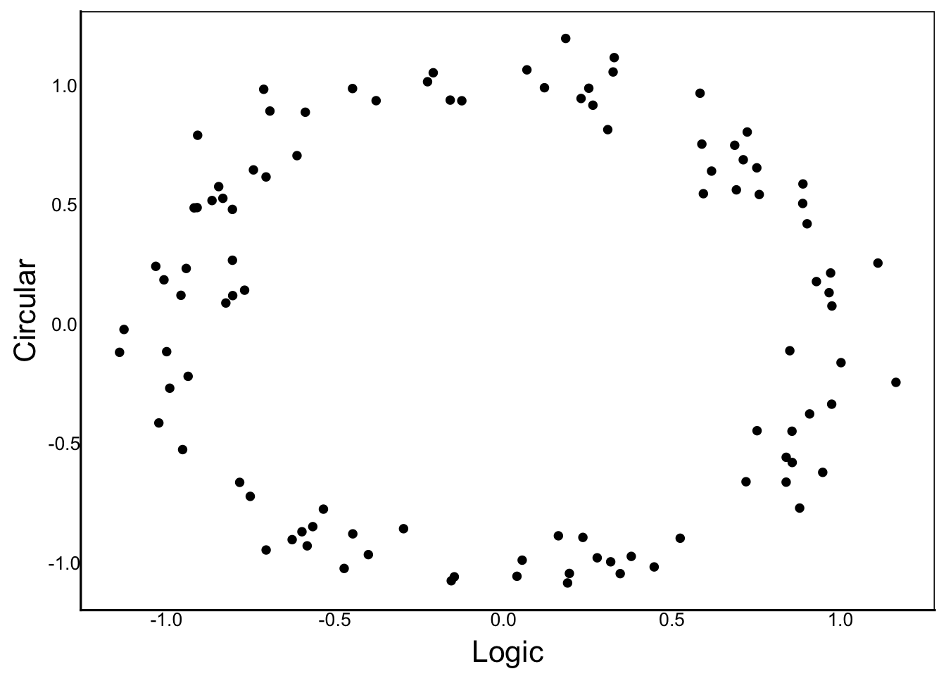
[1] "Product-Moment Correlation: -0.018"

[1] "Rank-Order Correlation: -0.018"

Detecting associations that are non-monotonic gets very tricky, because there are many possible relationships to explore.

These methods typically use resampling or permutation tests, which are computational methods that are beyond the scope of this book. Watch for a future book in the R Crash Course series to cover this some time in 2024 or 2025. Towards the end of this book, you will be introduced to Generalized Additive Models, which provide methods for exploring some non-monotonic relationships.

In the meantime, you can try to use data transformations to deal with non-monotonic relationships. In biological data, transforming one or both of your x and y axes with log() or exp() will often get you close to a linear relationship. You can use simple bivariate visualizations to explore how these transformations affect the apparent relationship between variables.

Normality Assumptions

Basic statistical models assume normality in the residuals; i.e. \(C_{skew}\) and \(C_{kurt}\) ~ 0. In the next chapter, we’ll explore this in more detail. In later chapters, we will explore models that use other distributions. But, even for basic linear models that violate normality assumptions, we can apply transformations to try to meet the model’s assumptions.

Tranformations

The first thing we can try are data transformations. A transformation is just an equation that we apply to the data to try to make it look more normal. The log-transformation is very common and often useful for this purpose. There is a fairly simple mathematical reason for this, if you remember that:

\[log(x*y) = log(x) + log(y)\]

Therefore, if our data are on an multiplicative or exponential scale, then a log-transformation puts them on a linear or additive scale.

ggplot() + geom_histogram(aes(x=log(ExpDat)))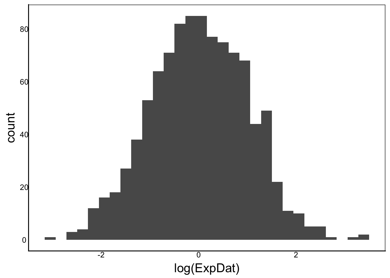

Moments(log(ExpDat))

[1] "Mean = 0"
[1] "Var = 1"
[1] "Cskew = 0"
[1] "Ckurt = 3"

ggplot() + geom_histogram(aes(x=log(multNorm)))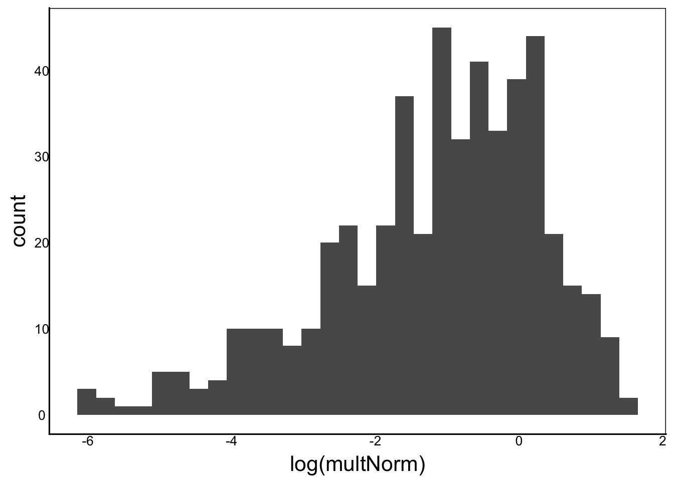

Moments(log(multNorm))

[1] "Mean = NaN"
[1] "Var = NA"
[1] "Cskew = NaN"
[1] "Ckurt = NaN"

ggplot() + geom_histogram(aes(x=log(invNorm)))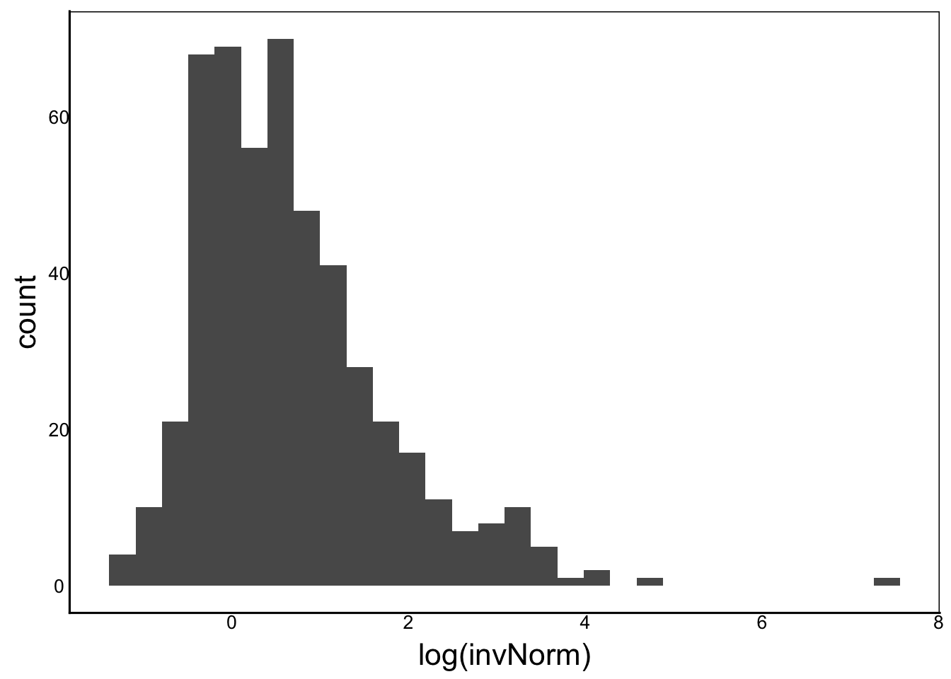

Moments(log(invNorm))

[1] "Mean = NaN"
[1] "Var = NA"
[1] "Cskew = NaN"
[1] "Ckurt = NaN"

ggplot() + geom_histogram(aes(x=log(BinDat)))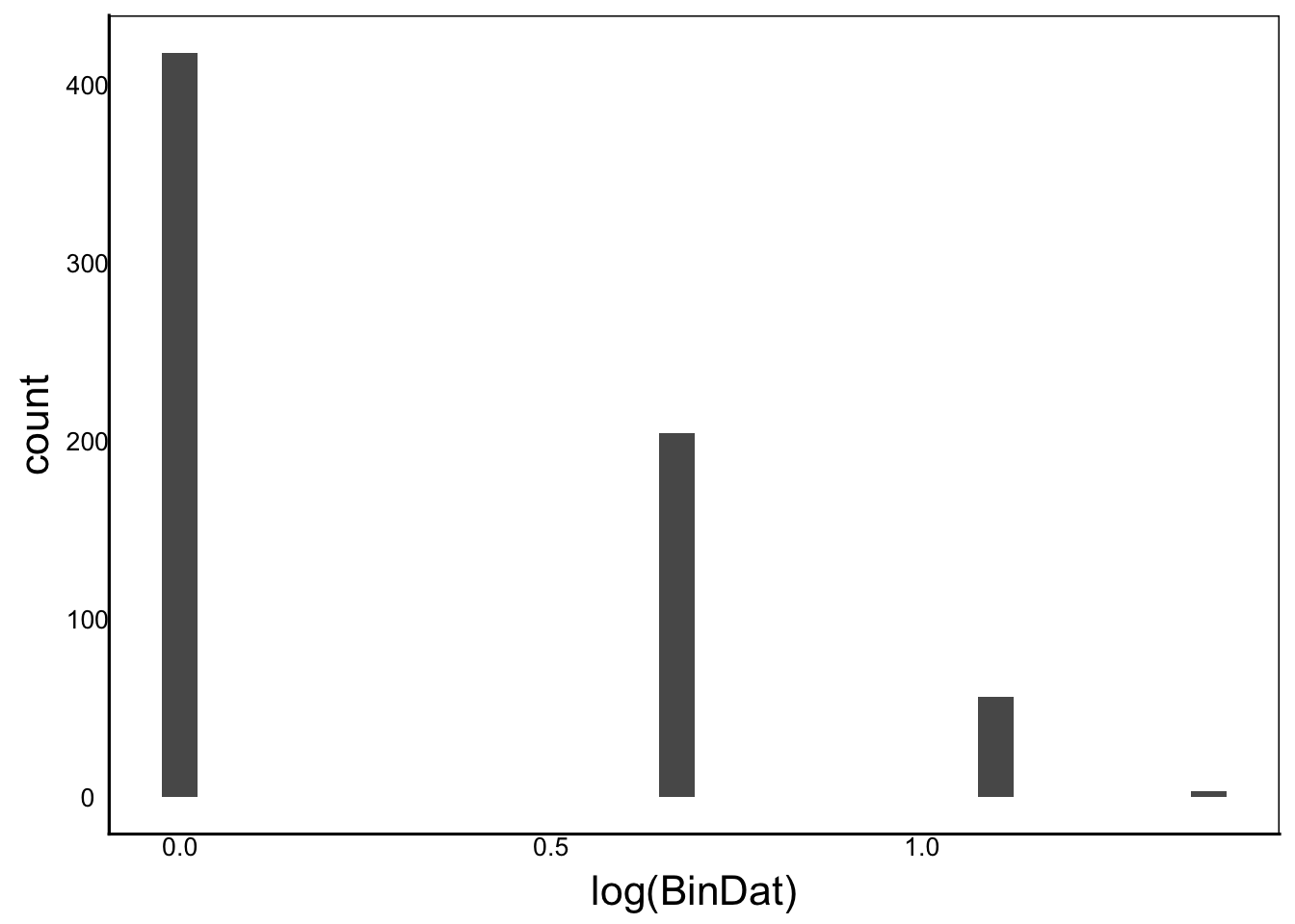

Moments(log(BinDat))

[1] "Mean = -Inf"
[1] "Var = NaN"
[1] "Cskew = NaN"
[1] "Ckurt = NaN"

ggplot() + geom_histogram(aes(x=log(PoisDat)))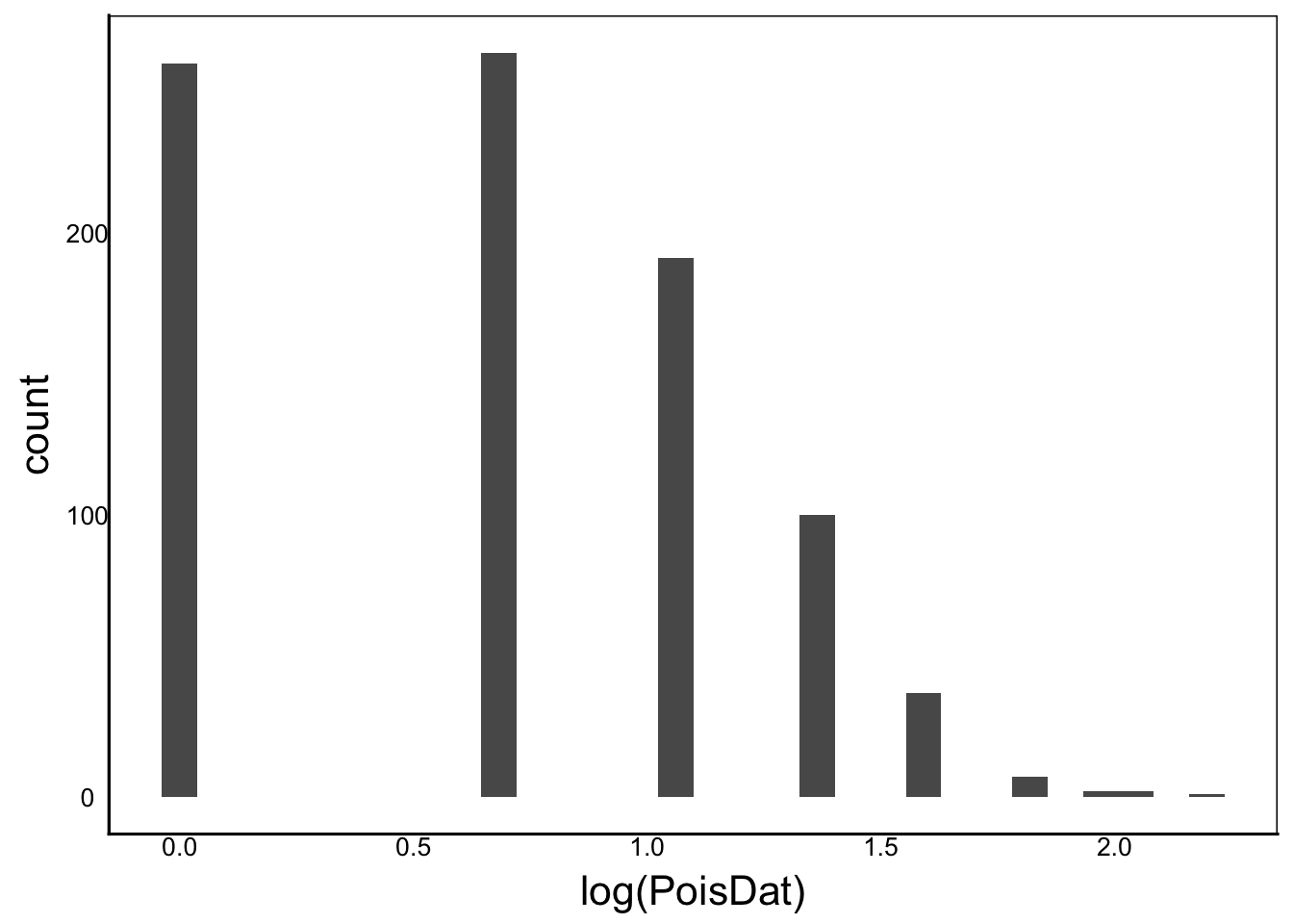

Moments(log(PoisDat))

[1] "Mean = -Inf"
[1] "Var = NaN"
[1] "Cskew = NaN"
[1] "Ckurt = NaN"

We still have a bit of skew in a couple of these but overall this is a big improvement. Even with the skew the data are much closer to normal than without the transformation.

Note in the output how the NaN and -Inf output from our Moments function. NaN occurs whenever we try to take the log of a negative number:

log(-10)

Warning in log(-10): NaNs produced

[1] NaN

and -Inf is the ‘value’ for the log of 0:

log(0)

[1] -Inf

But not ALL of the input data are like this. Why do we get the output for of NaN or -Inf for a vector that includes the log of positive values greater than zero?

The reason is similar to what we see with functions like mean() and sd() that include vectors with NA. As with missing values, we can use na.rm=T in these functions to run the calculations only on the values of the vector that are not NA, NaN or -Inf

X<-c(1,0,1,NaN,-Inf)
mean(X)

[1] NaN

mean(X,na.rm=T)

[1] -Inf

We could modify our Moments function to include na.rm=T in all of the individual functions that would return an NA, NaN or -Inf value.

Another common transformation is the square-root transformation:

ggplot() + geom_histogram(aes(x=sqrt(ExpDat)))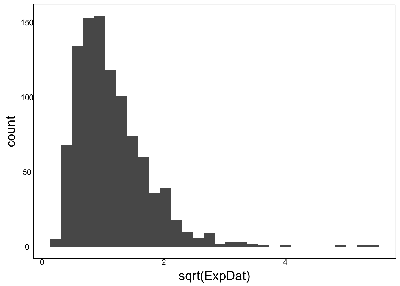

ggplot() + geom_histogram(aes(x=sqrt(multNorm)))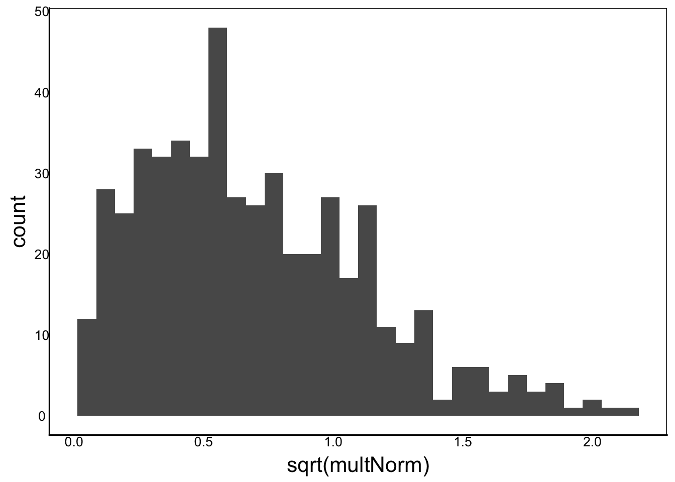

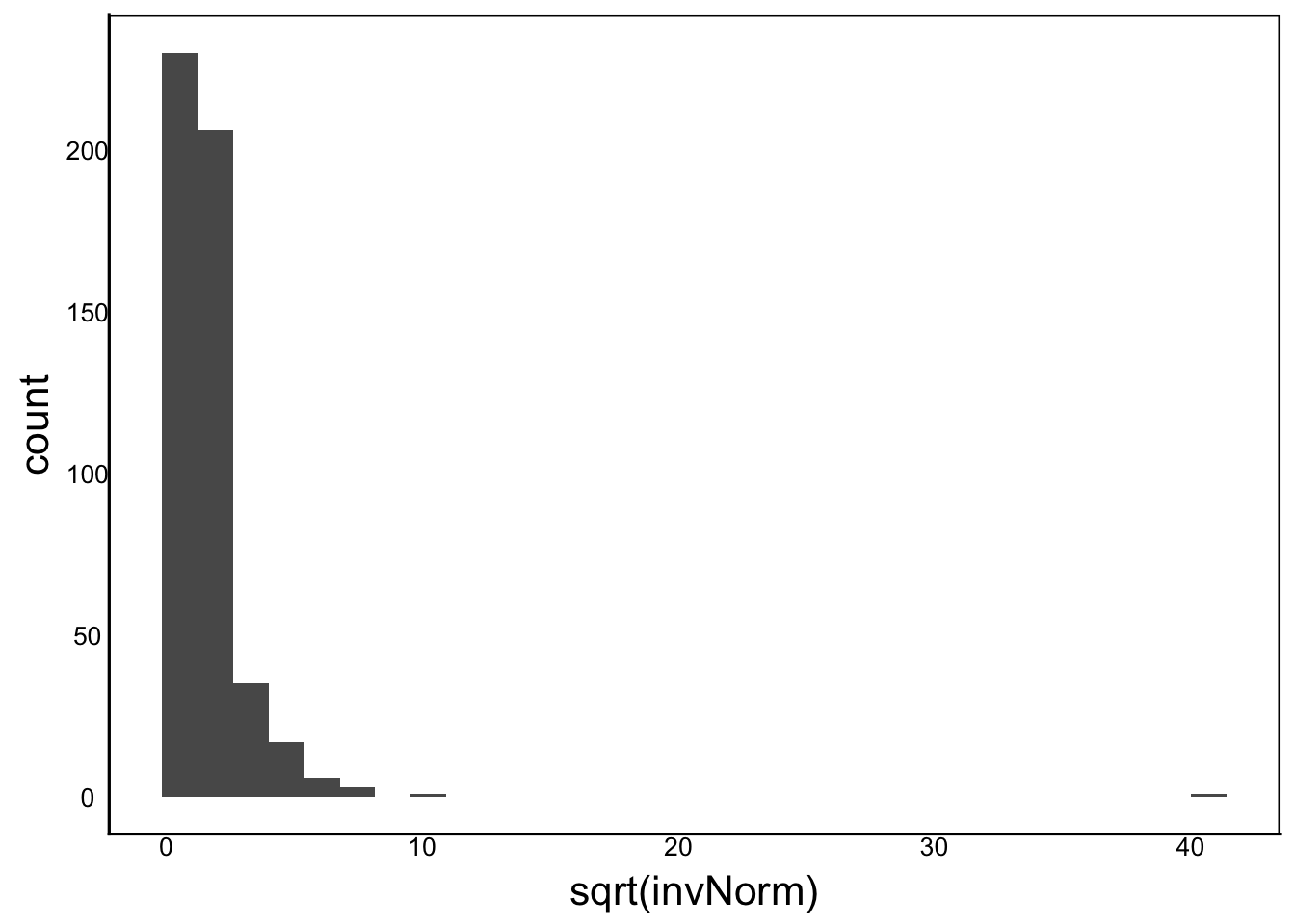
ggplot() + geom_histogram(aes(x=sqrt(invNorm)))