Model Selection

Introduction

In previous chapters, we have seen how each linear model represents a specific hypothesis defined by the variables input into the model. By convention, we reject the null hypothesis in favour of the alternative hypothesis. In the Advanced Linear Models Chapter we looked at some of the problems with this approach. First, we have the problem of false-positives (aka Type I error) is amplified by our desire to have a relatively conservative criteria for rejecting the null (p < 0.05). The Type I error occurs when we fail to reject the null hypothesis even though it is false. For example, if we find no significant effect of a new drug but in reality the drug has a effect. These errors are amplified because most studies that fail to reject a null do not ever get published. Another problem is the false discovery rate (FDR). If we test a bunch of different models, we will reject the null ‘just by chance’ about 5% of the time.

But there is another way to think about statistical hypotheses. Instead of having a simple true/false or pass/fail or significant/non-significant binary outcome, we can take a different approach that tests among hypotheses using model selection. In this case we are testing among many different alternative hypotheses instead of just rejecting (or failing to reject) a single hypothesis.

Although these represent different philosophies, in practice the difference usually comes down to the type of data. The ‘classic’ approach of null hypothesis testing is common in experiments with smaller sample sizes and a few, tightly controlled variables. Model selection is more common in large datasets with many observations and many potential predictor variables. A simple laboratory or greenhouse experiment with just one or two treatments would be a good example of this.

Setup

Load libraries and custom plotting theme

library(ggplot2) # plotting library

Warning: package 'ggplot2' was built under R version 4.5.2

library(dplyr) # data management

# Set custom plotting theme
source("http://bit.ly/theme_pub") 
theme_set(theme_pub())

We are also going to use two new libraries: lmtest for our linear model testing and MuMIn for Multi Model Inference and model selection. We also use MASS from the 2002 book Modern Applied Statistics with S. S is another programming language that R is based on. Don’t forget to use install.packages() to update/install these before you load the library() for the first time.

library(lmtest)

Loading required package: zoo

Warning: package 'zoo' was built under R version 4.5.2

Attaching package: 'zoo'

The following objects are masked from 'package:base':

    as.Date, as.Date.numeric

library(MuMIn)

Warning: package 'MuMIn' was built under R version 4.5.2

library(MASS)

Attaching package: 'MASS'

The following object is masked from 'package:dplyr':

    select

Model Selection

So far, we have framed linear models in terms of null vs alternative hypotheses. But there are some problems with this approach, including the False Discovery problem and a few others outlined in a nice YouTube video from Queen’s Alumn Veritasium (https://youtu.be/42QuXLucH3Q), and in this paper by John Ioannidis in PLoS Medicine (https://journals.plos.org/plosmedicine/article?id=10.1371/journal.pmed.0020124).

An alternate approach to running multiple independent models is to simultaneously test multiple models to see which one is best supported by the data or if several are equally-well supported. Each model represents a different hypothesis, so model selection is a way to test among alternative hypotheses, rather than just testing a series of single hypotheses against the null.

Goodness-of-Fit

In order to select among models, we need some metric that describes how well each model describes (or predicts) the data. These are known as fit or goodness-of-fit, and there are three main classes: \(R^2\), Likelihood, and Information Criteria.

\(R^2\)

We have already seen this in our linear model outputs. The \(R^2\) value ranges from 0 to 1 and describes how well the data fit the prediction. Let’s look at two examples:

X<-rnorm(100)
Y1<-rnorm(100)+0.3*X
Y2<-X

pDat<-as.data.frame(cbind(X,Y1,Y2))

ggplot(aes(x=X,y=Y1), data=pDat)+
  geom_point() + 
  geom_smooth(method="lm")

`geom_smooth()` using formula = 'y ~ x'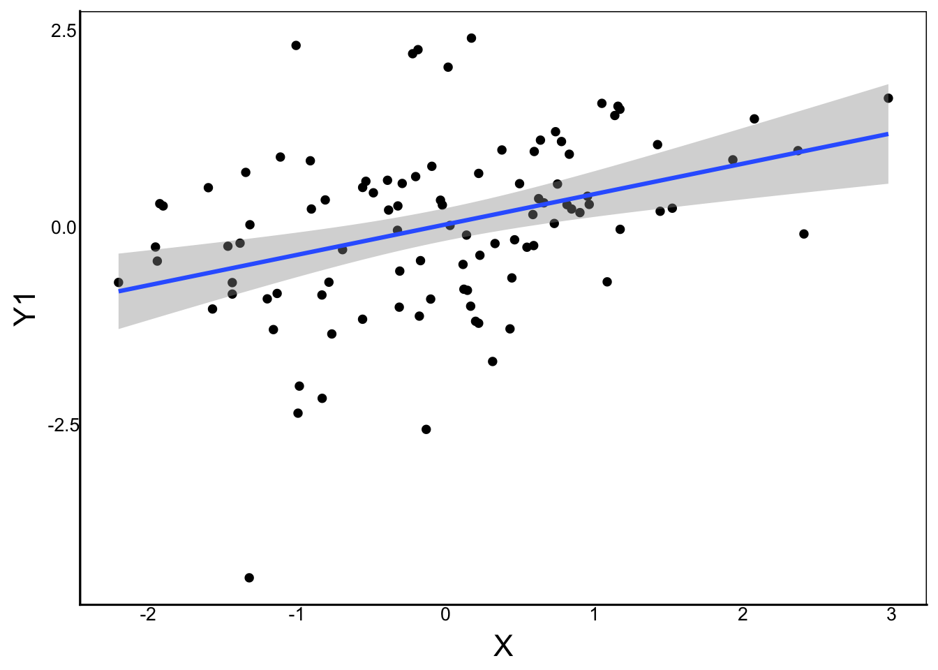

Rmod1<-lm(Y1~ X)
summary(Rmod1)

Call:
lm(formula = Y1 ~ X)

Residuals:
    Min      1Q  Median      3Q     Max 
-3.9709 -0.4968  0.0212  0.6456  2.6578 

Coefficients:
            Estimate Std. Error t value Pr(>|t|)    
(Intercept)  0.03319    0.10380    0.32  0.74983    
X            0.38547    0.10011    3.85  0.00021 ***
---
Signif. codes:  0 '***' 0.001 '**' 0.01 '*' 0.05 '.' 0.1 ' ' 1

Residual standard error: 1.038 on 98 degrees of freedom
Multiple R-squared:  0.1314,    Adjusted R-squared:  0.1225 
F-statistic: 14.83 on 1 and 98 DF,  p-value: 0.0002104

ggplot(aes(x=X,y=Y2), data=pDat)+
  geom_point() + 
  geom_smooth(method="lm")

`geom_smooth()` using formula = 'y ~ x'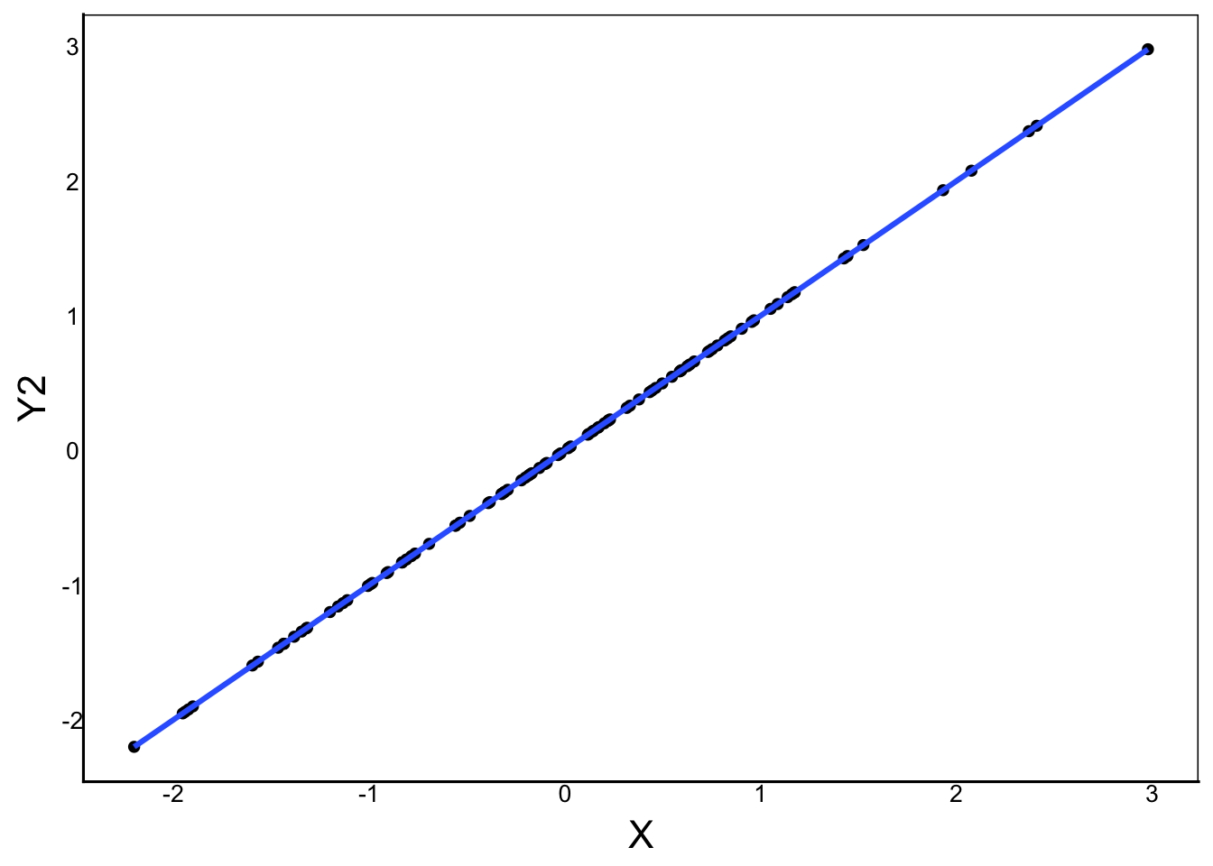

Rmod2<-lm(Y2 ~ X)
summary(Rmod2)

Call:
lm(formula = Y2 ~ X)

Residuals:
       Min         1Q     Median         3Q        Max 
-2.253e-16 -2.394e-17 -7.350e-18  1.582e-17  6.291e-16 

Coefficients:
             Estimate Std. Error   t value Pr(>|t|)    
(Intercept) 0.000e+00  7.934e-18 0.000e+00        1    
X           1.000e+00  7.652e-18 1.307e+17   <2e-16 ***
---
Signif. codes:  0 '***' 0.001 '**' 0.01 '*' 0.05 '.' 0.1 ' ' 1

Residual standard error: 7.931e-17 on 98 degrees of freedom
Multiple R-squared:      1, Adjusted R-squared:      1 
F-statistic: 1.708e+34 on 1 and 98 DF,  p-value: < 2.2e-16

Note that \(R^2\) is bounded between 0 (no fit) and 1 (perfect fit).

More specifically, the \(R^2\) is the squared correlation between the predicted and the residuals of the model:

cor(predict(Rmod1),Y1)^2

[1] 0.1314002

cor(predict(Rmod2),Y2)^2

[1] 1

Notice that the first one is slightly different from the Adjusted R-squared, because the Adjusted corrects for random correlations that arise by chance. As sample size increases, the Adjusted R-squared approaches the actual R-squared (i.e. squared correlation).

ANOVA

If we have two tests that are nested then we can calculate an ANOVA on the residual sums of squares. Nested just means that one model is a subset of the other. In the following example, ModB is nested within ModA, and ModC is nested in both ModB and ModA:

ModA<-lm(Y ~ X1 + X2 + X1:X2)
ModB<-lm(Y ~ X1 + X2)
ModC<-lm(Y ~ X1)

In contrast, this model would not be nested because it contains a predictor that isn’t found in the other models:

ModD<-lm(Y ~ X1 + X2 + X3)

We can test nested linear models using the anova function in R, which tests the hypothesis that the larger or full model fits the data better than the smaller or reduced model. Here’s a simple example:

X1<-rnorm(1000)
X2<-rnorm(1000)
Y<-X + X2 + rnorm(1000)
Full<-lm(Y ~ X1 + X2)
Reduced<-lm(Y ~ X1)

Now, we can ask:

Does the Full model fit the data better than the reduced model?

OR

Does adding predictor \(X2\) improve the model more than we would expect by chance?

Note that these questions are statistically equivalent, even though the wording is the reversed (removing vs adding a predictor).

anova(Reduced,Full)

Analysis of Variance Table

Model 1: Y ~ X1
Model 2: Y ~ X1 + X2
  Res.Df    RSS Df Sum of Sq      F    Pr(>F)    
1    998 3342.1                                  
2    997 2196.0  1      1146 520.31 < 2.2e-16 ***
---
Signif. codes:  0 '***' 0.001 '**' 0.01 '*' 0.05 '.' 0.1 ' ' 1

Note that this is an ANOVA with degrees of freedom equal to the difference in the number of parameters (1 regression coefficient in this case).

Likelihood & LRT

The likelihood of a model is a mathematical description of the probability that a given statistical model could produce the observed data. We typically use the theta symbol (\(\theta\)) to denote the likelihood, which is a value between 1 and 0. Unlike \(R^2\), each likelihood value is unique to a model and the dataset on which it is tested. Models fit to larger datasets will have smaller likelihoods than smaller datasets, but that doesn’t mean the model is less probable.

We can only compare likelihoods for different models tested on the same data.

One way to compare models is the Likelihood Ratio Test (LRT). The LRT gets its name from the statistic:

\[-2\ln(\frac{\theta_0}{\theta_1})\]

Where \(\theta\) is the likelihood of a model, and the subscripts 0 and 1 are for two nested models. The model with less parameters goes in the numerator, and the model with more parameters goes in the denominator

The likelihood of the model (\(\theta\)) is quite complicated, but for now just understand the model: Know that you can calculate the likelihood of any model by taking the natural log of the ratio of the two likelihoods (one from each model), and then multiplying by negative 2 gives you the likelihood ratio. You can test this value against a \(\chi^2\) distribution, with degrees of freedom equal to the difference in the degrees of freedom (number of predictors).

Thus, the LRT is very similar to the anova function for linear models, except that the LRT uses the \(\chi^2\) distribution of likelihoods whereas the anova function in R uses the \(F\)-distribution of variances.

Information Criteria

Information criteria are another set of statistics that measure the fit of a model to the data. An important distinction from the other metrics is that there is no statistical test, and no p-values associated with information criteria. You just compare the information criteria of different models to find the best one.

AIC

The most common information criterion is the Akike Information Criterion or AIC. The mathematical definition of AIC is:

\[ AIC = -2 [\ln(\theta)-k]\]

which is the same as

\[ AIC = 2k - 2 \ln(\theta)\]

where \(k\) is the number of parameters in the model, and \(ln(\theta)\) is the natural log of the likelihood of the model. Yes, the same likelihood as the Likelihood Ratio Test (LRT)!

The ‘best’ model is the one with the lowest AIC

Unlike the LRT, there is no p-value associated with AIC. Instead, we can compare the information criteria of models to see compare how well each fits the data. We calculate the absolute value of the difference in AIC between the better model (lower AIC) and the worse model (higher AIC):

\[\Delta_{AIC} = |AIC_{better} - AIC_{worse}|\]

where \(AIC_{better}\) is the model with the lower AIC (i.e. better fit to the data), and \(AIC_{worse}\) is the model with the higher AIC.

There is a rule of thumb for information criteria that is analogous to \(p\)-values. Two or more models are considered ‘equivalent’ if the difference in AIC between the models is less than 2. We can also calculate something analogous to the log-likelihood ratio for the LRT. The relative likelihood of two models is:

\[ e^{1/2 (AIC_{better} - AIC_{worse})} \]

The value will be between zero (large difference) and 1 (no difference). For example, if we had AIC values of \(AIC_1 = 25\) and \(AIC_2 = 38\), our relative likelihood would be:

\[ e^{1/2(25-38)} = 0.001503439\]

We would say that the model for \(AIC_2\) is 0.15% as probable as \(AIC_1\). Meaning, that \(AIC_1\) is a much better fit to the data. Our rule of thumb of \(\Delta AIC = 2\) for comparing models translates to:

\[ e^{1/2(-2)} = e^{-1} = 0.36\] or about 1/3 as probable. This is less stringent than our \(P < 0.05\) threshold for our likelihood ratio test, which corresponds to:

\[\ln(0.05)=e^{-2.996}\]

which we can round to a \(\Delta AIC\) of 3. In other words, a \(\Delta AIC\) greater than 3 corresponds to a worse model that is 5% as likely as the better model, analogous to \(P < 0.05\) in the likelihood ratio test.

AICc

Another common and important criterion is AICc. This is just the AIC with an equation added to adjust for small sample datasets.

\[AICc = AIC +{\frac {2k^{2}+2k}{n-k-1}} \]

Where \(n\) is the sample size. As \(n\) increases, the denominator of the second term moves toward zero. So as sample size increases, AICc approaches AIC. Note also that \(k\) is in the denominator too, so we need larger sample sizes when including more complicated models.

BIC

The Bayes Information Criterion or BIC is related to Bayes’ theorem. It is similar to AICc but with a different adjustment for sample size:

\[ {BIC} =k\ln(n)-2\ln(\theta) \] as above, \(n\) denotes samples size, \(k\) the number of parameters estimated in the model, and \(\theta\) is the likelihood of the model.

CAUTION: Missing Values

In addition to the usual assumptions of linear models, a very important quality check for model selection is to make sure that each model has the exact same number of observations. For our simulated data it’s no problem, but with real data you may be missing observations for certain predictor variables. In that case, you will have different data in models that include or exclude predictor variables with one or more missing values.

A really simple way to deal with this is to make a dataset containing ONLY the predictor and response variables you want to use in model selection, and then use the complete.cases function to remove any rows with missing values.

Here’s an example:

Incomplete<-data.frame(A = c(0,1,2,3,4,5),
                       B = c(0,1,NA,3,4,5),
                       C = c(0,1,2,3,NA,5))

Incomplete

  A  B  C
1 0  0  0
2 1  1  1
3 2 NA  2
4 3  3  3
5 4  4 NA
6 5  5  5

Our incomplete data.frame has 6 rows

Which rows have complete data?

complete.cases(Incomplete)

[1]  TRUE  TRUE FALSE  TRUE FALSE  TRUE

Remove rows with missing data:

Incomplete %>%
  filter(complete.cases(Incomplete))

  A B C
1 0 0 0
2 1 1 1
3 3 3 3
4 5 5 5

From this example, you can see an important limitation of model selection: If we have many predictors, and each has a few missing observations, we lose ALL of the rows with AT LEAST one missing value. This can quickly shrink our dataset and reduce our statistical power (e.g. from 6 rows to 4 in the above example).

Impute Missing Data

One approach to dealing with missing observations is to impute the missing values. An imputation is a mathematical ‘guess’ of what the likely value would be. This works only if missing data are sparse (i.e. few) and random – that is, there aren’t too many NA values, and they are randomly distributed across rows and columns. Imputation methods are covered in the R Intro to Machine Learning textbook.

Model Selection Examples

Now that you know the math, let’s try some examples.

LRT

The Likelihood Ratio Test (LRT) compares the likelihood of two models. The likelihood ratio statistic follows a chi-squred distribution with degrees of freedom equal to the difference in the number of parameters.

To run a likelihood ratio test, we can use a function from the lmtest library

library(lmtest)

Let’s run an example with completely random numbers but different number of predictors, then we run the LRT using the lrtest function:

Y<-rnorm(1000)
X1<-rnorm(1000)
X2<-rnorm(1000)
X3<-rnorm(1000)
Mod1<-lm(Y ~ X1 + X2 + X3)
Mod2<-lm(Y ~ X1)
lrtest(Mod2,Mod1)

Likelihood ratio test

Model 1: Y ~ X1
Model 2: Y ~ X1 + X2 + X3
  #Df  LogLik Df  Chisq Pr(>Chisq)
1   3 -1428.4                     
2   5 -1428.0  2 0.8517     0.6532

Now run the above code a bunch of times and compare the output.

Each time we get the same number of degrees of freedom (#Df): 5 in model 2 and 3 in model 1. We get the same difference in degrees of freedom (Df) of 2 because there are 2 more predictors in Mod1 than Mod2.

The Chisq is -2 times the \(ln\) of the ratio of the LogLik values. We can then calculate the probability from the chi-square distribution. For example, if we have 1.09 in our Chisq above, with 2 df for the difference in parameters:

pchisq(q=1.09,df=2, lower.tail=F)

[1] 0.5798418

The LogLik is the natural-log-scaled likelihood of the model. The likelihood describes how well the data fit the model (how likely is the model given the data), so the specific likelihood depends on the scatter of points around the prediction of the model (in this case, a single or multiple regression). The Likelihood is a probability. Specifically, it’s the probability you would observe these exact data if the model is true. So if the LogLik is -120, then the likelihood of the model is the exponential \(e^{-120}\), or approximately:

\[0.00000000000000000000000000000000000000000000000000767 \]

That’s a very small probability! But that doesn’t mean that the model is unlikely. It’s the same probability you might get if you flip a coin 1000 times and ask: “what’s the probability you would get EXACTLY 500 heads and 500 tails?”

Question: What is the probability of getting exactly 4 heads with 4 coin tosses?

Answer: There are \(2^4\) possible outcomes, but only 1 way to get 4 heads, therefore:

\(P(4 heads) = \frac{1}{2^4} = 0.625\)

We can also calculate this using the density function.

dbinom(4,size=4,prob=0.5)

[1] 0.0625

Note that the probability is much larger. Any specific outcome becomes less likely as the sample size increases, but that doesn’t mean the model is wrong! That’s why we have to compare probabilities. We only have 1 set of observations (Y), but we can ask the probability of observing that data for any given statistical model.

Of course in this case, we also get a low likelihood of the model because we are choosing random variables with no association.

NOTE: Why do we use a natural-log scale?

The main reason is that computers are not very good at working with small numbers. For example:

exp(-1)

[1] 0.3678794

exp(-10)

[1] 4.539993e-05

exp(-100)

[1] 3.720076e-44

exp(-1000)

[1] 0

Note that \(e^{-1000}\) is a very small number, but it’s not zero!

The problem is with the way computer memory stores very small numbers. To avoid working with very small fracitons, we use log-likelihood instead of raw likelihood. Taking the log of a very small number changes it from a tiny fraction to a large integer, which is much easier for computer memory to work with. And since we know that:

1. The probability of two independent events A and B is \(P(A)\times P(B)\)
2. \(log(A\times B) = log(A) + log(B)\)

We can work with complicated models by adding log-likelihoods instead of multiplying raw likelihoods.

AICc & BIC

We can similarly compare models with information criteria using AIC

AIC(Mod1)

[1] 2866.007

AIC(Mod2)

[1] 2862.859

AIC(Mod1) - AIC(Mod2)

[1] 3.148259

and we can convert this to a probability.

exp(0.5*AIC(Mod2)-0.5*AIC(Mod1))

[1] 0.2071878

The smaller model (Mod2) is about 15% as likely as the larger model (Mod1)

Likewise, we can do model selection with BIC:

BIC(Mod1)

[1] 2890.546

BIC(Mod2)

[1] 2877.582

BIC(Mod1) - BIC(Mod2)

[1] 12.96377

Remember the basic rule of thumb is that models are equivalent if their delta (difference in AIC or BIC) is less than 2. If the difference is bigger than 2, then we choose the model with the smaller AIC or BIC.

Try re-running the code to randomly generate the variables above, then re-run the LRT, AIC and BIC to compare the results. How often do you get a non-signifcant LRT but a delta AIC or BIC bigger than 2?

Now that we’ve simulated an example to compare the two main approaches for model fitting and model selection, let’s look at some automated methods.

Model Selection Functions

Forward Selection

With forward selection you add variables one at a time and compare the fit of the model to decide if the predictor should stay in the model in the next round. Typically, we might:

1. Start with the most basic model
2. Do a model selection with each term on its own
3. Add the term with the model that fits best
4. Repeat until no terms improve the fit of the model

Backward Selection

Backward selection starts with all of the variables in the model and then removes predictors one at a time to test the fit of the model. In biological studies with a few nested models, this is a commonly done using the LRT.

1. Put all parameters in the model
2. Remove one parameter at a time, starting with the most complex interaction term(s)
3. If you are using Information Criteria, keep the model with lower score (better fit)
   • If you are using the LRT then keep the parameter in only if the LRT is significant (i.e. leaving the parameter in the model is a significantly better fit)
4. Important: If an interaction is significant, then ALL of the individual terms in the interaction should also be retained in the model. For example, if \(A:B\) is significant, then we must keep all three terms in the model (\(A + B + A:B\)), even if the estimates for \(A\) or \(B\) (or both) are non-significant when included in the model with \(A:B\).

Dredging

This is a general term for comparing many models. The idea is you are running your statistical tool through the muck of models to find something valuable. If you have many predictor variables you would not typically include interaction terms because this would greatly increase the number of models you would have to test. As you can imagine, the more models you test the more likely you are to find a spurious relationship. Nevertheless, this can be a powerful approach as long as you are careful about interpretation (e.g. run follow-up experiments to test significant relationships). If you have a large dataset, you can split it into a ‘training’ dataset and a ‘validation’ dataset. In this case, you would dredge the training dataset and then validate the model on the validation dataset. This is a common approach in machine learning and is covered in the R Intro to Machine Learning Book.

Examples

The MuMIn and MASS packages in R have some convenient functions for running model selection

library(MuMIn)
library(MASS)

We will try these different approaches on the FallopiaData.csv, which is available for download here: https://colauttilab.github.io/RCrashCourse/FallopiaData.csv. These are plant biomass data for different species competing in pots.

InDat<-read.csv(
  "https://colauttilab.github.io/RCrashCourse/FallopiaData.csv")
str(InDat)

'data.frame':   123 obs. of  13 variables:
 $ PotNum      : int  1 2 3 5 6 7 8 9 10 11 ...
 $ Scenario    : chr  "low" "low" "low" "low" ...
 $ Nutrients   : chr  "low" "low" "low" "low" ...
 $ Taxon       : chr  "japon" "japon" "japon" "japon" ...
 $ Symphytum   : num  9.81 8.64 2.65 1.44 9.15 ...
 $ Silene      : num  36.4 29.6 36 21.4 23.9 ...
 $ Urtica      : num  16.08 5.59 17.09 12.39 5.19 ...
 $ Geranium    : num  4.68 5.75 5.13 5.37 0 9.05 3.51 9.64 7.3 6.36 ...
 $ Geum        : num  0.12 0.55 0.09 0.31 0.17 0.97 0.4 0.01 0.47 0.33 ...
 $ All_Natives : num  67 50.2 61 40.9 38.4 ...
 $ Fallopia    : num  0.01 0.04 0.09 0.77 3.4 0.54 2.05 0.26 0 0 ...
 $ Total       : num  67.1 50.2 61.1 41.7 41.8 ...
 $ Pct_Fallopia: num  0.01 0.08 0.15 1.85 8.13 1.12 3.7 0.61 0 0 ...

WARNING: There are several columns that are calculated from other columns. Including everything will give us problems due to collinearity, which is covered in the Advanced Linear Models Chapter.

In particular, these columns should be excluded from the model selection:

• All_Natives
• Total
• Pct_Fallopia

Forward Selection

Let’s see how well we can predict total biomass. We already know that this is calculated as the sum of all other plant biomasses, so to prevent co-linearity we will only look at the biomass of the native plants (i.e. exclude Fallopia and the treatment columns).

The first step is to specify the full model. We’ll add in a random variable

set.seed(4567)
InDat$RAND<-rnorm(nrow(InDat))
MinMod<-lm(Total ~ 1, data=InDat)
FullMod<-lm(Total ~ Symphytum + Silene + Urtica + Geranium + Geum 
            + RAND, data=InDat)

Then we can use the stepAIC function for stepwise selection using AIC

ForSel<-stepAIC(MinMod, scope=formula(FullMod), 
                direction="forward")

Start:  AIC=565.9
Total ~ 1

            Df Sum of Sq     RSS    AIC
+ Silene     1   2772.24  9276.4 535.73
+ Urtica     1   1545.26 10503.4 551.01
+ Geum       1    510.16 11538.5 562.58
<none>                   12048.7 565.90
+ Geranium   1    187.22 11861.5 565.97
+ RAND       1    104.30 11944.4 566.83
+ Symphytum  1     77.31 11971.4 567.10

Step:  AIC=535.73
Total ~ Silene

            Df Sum of Sq    RSS    AIC
+ Urtica     1    3710.1 5566.3 474.91
+ Geranium   1    1012.1 8264.3 523.52
+ Geum       1     641.9 8634.5 528.91
+ Symphytum  1     155.3 9121.1 535.66
<none>                   9276.4 535.73
+ RAND       1      80.9 9195.5 536.66

Step:  AIC=474.91
Total ~ Silene + Urtica

            Df Sum of Sq    RSS    AIC
+ Geranium   1   1575.16 3991.1 436.00
+ Symphytum  1   1211.04 4355.2 446.74
+ Geum       1    116.07 5450.2 474.32
+ RAND       1     91.44 5474.8 474.88
<none>                   5566.3 474.91

Step:  AIC=436
Total ~ Silene + Urtica + Geranium

            Df Sum of Sq    RSS    AIC
+ Symphytum  1   1251.40 2739.7 391.72
+ Geum       1     88.35 3902.8 435.24
<none>                   3991.1 436.00
+ RAND       1     19.85 3971.3 437.38

Step:  AIC=391.72
Total ~ Silene + Urtica + Geranium + Symphytum

       Df Sum of Sq    RSS    AIC
+ Geum  1    58.681 2681.1 391.06
<none>              2739.7 391.72
+ RAND  1     2.087 2737.7 393.63

Step:  AIC=391.06
Total ~ Silene + Urtica + Geranium + Symphytum + Geum

       Df Sum of Sq    RSS    AIC
<none>              2681.1 391.06
+ RAND  1     2.797 2678.3 392.93

From the output, we can see the AIC for each model, and go down until the difference is < 2. We can also do a regular linear model of the ‘best’ model if we want a more conventional statistical analysis. The advantage here is that we only run the statistical analysis on the ‘best’ model.

summary(ForSel)

Call:
lm(formula = Total ~ Silene + Urtica + Geranium + Symphytum + 
    Geum, data = InDat)

Residuals:
   Min     1Q Median     3Q    Max 
-7.984 -2.910 -1.171  1.280 18.493 

Coefficients:
            Estimate Std. Error t value Pr(>|t|)    
(Intercept) 12.21815    2.47000   4.947 2.55e-06 ***
Silene       0.80007    0.04441  18.015  < 2e-16 ***
Urtica       0.92486    0.06397  14.457  < 2e-16 ***
Geranium     0.90367    0.10843   8.334 1.72e-13 ***
Symphytum    0.76473    0.10473   7.302 3.73e-11 ***
Geum         1.93416    1.20866   1.600    0.112    
---
Signif. codes:  0 '***' 0.001 '**' 0.01 '*' 0.05 '.' 0.1 ' ' 1

Residual standard error: 4.787 on 117 degrees of freedom
Multiple R-squared:  0.7775,    Adjusted R-squared:  0.768 
F-statistic: 81.76 on 5 and 117 DF,  p-value: < 2.2e-16

Backward Selection

It’s trivial to adapt the code above for backward selection; we use the same model but a different direction:

BackSel<-stepAIC(FullMod, direction="backward")

Start:  AIC=392.93
Total ~ Symphytum + Silene + Urtica + Geranium + Geum + RAND

            Df Sum of Sq     RSS    AIC
- RAND       1       2.8  2681.1 391.06
<none>                    2678.3 392.93
- Geum       1      59.4  2737.7 393.63
- Symphytum  1    1202.5  3880.7 436.55
- Geranium   1    1546.4  4224.7 446.99
- Urtica     1    4771.9  7450.2 516.77
- Silene     1    7342.2 10020.5 553.23

Step:  AIC=391.06
Total ~ Symphytum + Silene + Urtica + Geranium + Geum

            Df Sum of Sq     RSS    AIC
<none>                    2681.1 391.06
- Geum       1      58.7  2739.7 391.72
- Symphytum  1    1221.7  3902.8 435.24
- Geranium   1    1591.7  4272.7 446.38
- Urtica     1    4789.6  7470.7 515.11
- Silene     1    7437.0 10118.0 552.42

summary(BackSel)

Call:
lm(formula = Total ~ Symphytum + Silene + Urtica + Geranium + 
    Geum, data = InDat)

Residuals:
   Min     1Q Median     3Q    Max 
-7.984 -2.910 -1.171  1.280 18.493 

Coefficients:
            Estimate Std. Error t value Pr(>|t|)    
(Intercept) 12.21815    2.47000   4.947 2.55e-06 ***
Symphytum    0.76473    0.10473   7.302 3.73e-11 ***
Silene       0.80007    0.04441  18.015  < 2e-16 ***
Urtica       0.92486    0.06397  14.457  < 2e-16 ***
Geranium     0.90367    0.10843   8.334 1.72e-13 ***
Geum         1.93416    1.20866   1.600    0.112    
---
Signif. codes:  0 '***' 0.001 '**' 0.01 '*' 0.05 '.' 0.1 ' ' 1

Residual standard error: 4.787 on 117 degrees of freedom
Multiple R-squared:  0.7775,    Adjusted R-squared:  0.768 
F-statistic: 81.76 on 5 and 117 DF,  p-value: < 2.2e-16

Forward + Backward

When there is some degree of collinearity in the predictors, then the Forward or Backward selection alone can miss the ‘best’ model because it only tests one predictor at a time.

We can combine methods for a more robust model testing.

BothSel<-stepAIC(MinMod, scope=formula(FullMod), 
                 direction="both")

Start:  AIC=565.9
Total ~ 1

            Df Sum of Sq     RSS    AIC
+ Silene     1   2772.24  9276.4 535.73
+ Urtica     1   1545.26 10503.4 551.01
+ Geum       1    510.16 11538.5 562.58
<none>                   12048.7 565.90
+ Geranium   1    187.22 11861.5 565.97
+ RAND       1    104.30 11944.4 566.83
+ Symphytum  1     77.31 11971.4 567.10

Step:  AIC=535.73
Total ~ Silene

            Df Sum of Sq     RSS    AIC
+ Urtica     1    3710.1  5566.3 474.91
+ Geranium   1    1012.1  8264.3 523.52
+ Geum       1     641.9  8634.5 528.91
+ Symphytum  1     155.3  9121.1 535.66
<none>                    9276.4 535.73
+ RAND       1      80.9  9195.5 536.66
- Silene     1    2772.2 12048.7 565.90

Step:  AIC=474.91
Total ~ Silene + Urtica

            Df Sum of Sq     RSS    AIC
+ Geranium   1    1575.2  3991.1 436.00
+ Symphytum  1    1211.0  4355.2 446.74
+ Geum       1     116.1  5450.2 474.32
+ RAND       1      91.4  5474.8 474.88
<none>                    5566.3 474.91
- Urtica     1    3710.1  9276.4 535.73
- Silene     1    4937.1 10503.4 551.01

Step:  AIC=436
Total ~ Silene + Urtica + Geranium

            Df Sum of Sq     RSS    AIC
+ Symphytum  1    1251.4  2739.7 391.72
+ Geum       1      88.3  3902.8 435.24
<none>                    3991.1 436.00
+ RAND       1      19.9  3971.3 437.38
- Geranium   1    1575.2  5566.3 474.91
- Urtica     1    4273.2  8264.3 523.52
- Silene     1    6320.8 10312.0 550.75

Step:  AIC=391.72
Total ~ Silene + Urtica + Geranium + Symphytum

            Df Sum of Sq     RSS    AIC
+ Geum       1      58.7  2681.1 391.06
<none>                    2739.7 391.72
+ RAND       1       2.1  2737.7 393.63
- Symphytum  1    1251.4  3991.1 436.00
- Geranium   1    1615.5  4355.2 446.74
- Urtica     1    5390.6  8130.4 523.51
- Silene     1    7550.3 10290.0 552.49

Step:  AIC=391.06
Total ~ Silene + Urtica + Geranium + Symphytum + Geum

            Df Sum of Sq     RSS    AIC
<none>                    2681.1 391.06
- Geum       1      58.7  2739.7 391.72
+ RAND       1       2.8  2678.3 392.93
- Symphytum  1    1221.7  3902.8 435.24
- Geranium   1    1591.7  4272.7 446.38
- Urtica     1    4789.6  7470.7 515.11
- Silene     1    7437.0 10118.0 552.42

Now we see many ‘base’ models showing how the fit changes as we add (+) or remove (-) from each base models.

summary(BothSel)

Call:
lm(formula = Total ~ Silene + Urtica + Geranium + Symphytum + 
    Geum, data = InDat)

Residuals:
   Min     1Q Median     3Q    Max 
-7.984 -2.910 -1.171  1.280 18.493 

Coefficients:
            Estimate Std. Error t value Pr(>|t|)    
(Intercept) 12.21815    2.47000   4.947 2.55e-06 ***
Silene       0.80007    0.04441  18.015  < 2e-16 ***
Urtica       0.92486    0.06397  14.457  < 2e-16 ***
Geranium     0.90367    0.10843   8.334 1.72e-13 ***
Symphytum    0.76473    0.10473   7.302 3.73e-11 ***
Geum         1.93416    1.20866   1.600    0.112    
---
Signif. codes:  0 '***' 0.001 '**' 0.01 '*' 0.05 '.' 0.1 ' ' 1

Residual standard error: 4.787 on 117 degrees of freedom
Multiple R-squared:  0.7775,    Adjusted R-squared:  0.768 
F-statistic: 81.76 on 5 and 117 DF,  p-value: < 2.2e-16

Interactions

Interactions add a lot of complexity to model fitting. Here’s an example with just four variables:

ComplexMod<-lm(Total ~ Symphytum*Silene*Urtica*RAND, 
               data=InDat)
CplxSel<-stepAIC(MinMod, scope=formula(ComplexMod), 
                 direction="both")

Start:  AIC=565.9
Total ~ 1

            Df Sum of Sq     RSS    AIC
+ Silene     1   2772.24  9276.4 535.73
+ Urtica     1   1545.26 10503.4 551.01
<none>                   12048.7 565.90
+ RAND       1    104.30 11944.4 566.83
+ Symphytum  1     77.31 11971.4 567.10

Step:  AIC=535.73
Total ~ Silene

            Df Sum of Sq     RSS    AIC
+ Urtica     1    3710.1  5566.3 474.91
+ Symphytum  1     155.3  9121.1 535.66
<none>                    9276.4 535.73
+ RAND       1      80.9  9195.5 536.66
- Silene     1    2772.2 12048.7 565.90

Step:  AIC=474.91
Total ~ Silene + Urtica

                Df Sum of Sq     RSS    AIC
+ Symphytum      1    1211.0  4355.2 446.74
+ RAND           1      91.4  5474.8 474.88
<none>                        5566.3 474.91
+ Silene:Urtica  1      40.1  5526.2 476.02
- Urtica         1    3710.1  9276.4 535.73
- Silene         1    4937.1 10503.4 551.01

Step:  AIC=446.74
Total ~ Silene + Urtica + Symphytum

                   Df Sum of Sq     RSS    AIC
+ Symphytum:Silene  1     319.5  4035.7 439.36
<none>                           4355.2 446.74
+ RAND              1      45.0  4310.2 447.46
+ Silene:Urtica     1      18.8  4336.4 448.20
+ Symphytum:Urtica  1       7.0  4348.2 448.54
- Symphytum         1    1211.0  5566.3 474.91
- Urtica            1    4765.9  9121.1 535.66
- Silene            1    6141.4 10496.6 552.93

Step:  AIC=439.36
Total ~ Silene + Urtica + Symphytum + Silene:Symphytum

                   Df Sum of Sq    RSS    AIC
+ Symphytum:Urtica  1      86.6 3949.2 438.70
<none>                          4035.7 439.36
+ RAND              1      31.0 4004.7 440.41
+ Silene:Urtica     1       2.6 4033.1 441.28
- Silene:Symphytum  1     319.5 4355.2 446.74
- Urtica            1    4681.4 8717.1 532.09

Step:  AIC=438.7
Total ~ Silene + Urtica + Symphytum + Silene:Symphytum + Urtica:Symphytum

                   Df Sum of Sq    RSS    AIC
<none>                          3949.2 438.70
+ Silene:Urtica     1     45.85 3903.3 439.26
+ RAND              1     44.42 3904.7 439.30
- Urtica:Symphytum  1     86.57 4035.7 439.36
- Silene:Symphytum  1    399.08 4348.2 448.54

summary(CplxSel)

Call:
lm(formula = Total ~ Silene + Urtica + Symphytum + Silene:Symphytum + 
    Urtica:Symphytum, data = InDat)

Residuals:
     Min       1Q   Median       3Q      Max 
-14.4483  -3.6256   0.0568   2.6176  20.4114 

Coefficients:
                 Estimate Std. Error t value Pr(>|t|)    
(Intercept)      11.18183    4.28716   2.608 0.010288 *  
Silene            1.00369    0.10427   9.626  < 2e-16 ***
Urtica            1.14232    0.18032   6.335 4.58e-09 ***
Symphytum         1.90793    0.37453   5.094 1.36e-06 ***
Silene:Symphytum -0.03638    0.01058  -3.439 0.000811 ***
Urtica:Symphytum -0.02870    0.01792  -1.602 0.111956    
---
Signif. codes:  0 '***' 0.001 '**' 0.01 '*' 0.05 '.' 0.1 ' ' 1

Residual standard error: 5.81 on 117 degrees of freedom
Multiple R-squared:  0.6722,    Adjusted R-squared:  0.6582 
F-statistic: 47.99 on 5 and 117 DF,  p-value: < 2.2e-16

Dredging

The dredge function from the MuMIn package is useful for testing all possible models. It has several additional parameters to help with model selection. An important one is beta=. This is a method for standardizing the beta (coefficients) estimates so that they can be compared across models.

ComplexMod<-lm(Total ~ Symphytum*Silene*Urtica*RAND, 
               data=InDat)
DMod<-dredge(ComplexMod, beta="sd")

Error in `dredge()`:
! 'global.model''s 'na.action' argument is not set and options('na.action') is "na.omit"

Note the error. This is an important warning about missing data. In our case, there are no missing data, but this error prevents us from accidentally comparing models with different numbers of observations. To run the model, we should set our global options to na.fail instead of na.omit:

options(na.action="na.fail")
DMod<-dredge(ComplexMod, beta="sd")

Fixed term is "(Intercept)"

head(DMod)

Global model call: lm(formula = Total ~ Symphytum * Silene * Urtica * RAND, data = InDat)
---
Model selection table 
     (Int)     RAN   Sln    Sym    Urt  RAN:Sym RAN:Urt Sln:Sym  Sln:Urt
208      0 -0.2744 1.202 0.7579 0.7024           0.2699 -0.4547         
9168     0 -0.2359 1.588 1.1870 1.4680           0.2154 -0.8123 -0.60830
720      0 -0.2576 1.240 0.8827 0.8412           0.2420 -0.4997         
976      0 -0.2599 1.324 0.9350 1.0270           0.2537 -0.5038 -0.13360
464      0 -0.2806 1.233 0.7466 0.7546           0.2843 -0.4431 -0.06766
240      0 -0.2404 1.206 0.7639 0.7016 -0.03178  0.2627 -0.4579         
     Sym:Urt Sln:Sym:Urt df   logLik  AICc delta weight
208                       8 -384.672 786.6  0.00  0.298
9168 -0.7120      0.4163 11 -381.541 787.5  0.85  0.194
720  -0.1635              9 -384.104 787.8  1.19  0.164
976  -0.2612             10 -383.195 788.4  1.75  0.124
464                       9 -384.391 788.4  1.77  0.123
240                       9 -384.630 788.9  2.25  0.097
Models ranked by AICc(x) 

The output include ALL of the models, so here we just look at the AICc, delta AICc and coefficients of the top models.

QA/QC

As always, we should inspect the residuals of the model to look for problems and test the assumptions as outlined in the Linear Models chapter. We also make sure there are no missing values in the columns used in our models.

Finally, we should also check the overall fit if our best model. The reason to do this is that there will always be a ‘best fit’ model in our model selection analysis, even if all the models are complete garbage. A good way to do this is to compare the prediction of the model against the observed values. The better the model, the more tightly the points will form a line with the observed values:

ggplot()+
  geom_point(aes(x=predict(Mod2), y=Y))+
  xlab("Predicted") + ylab("Observed")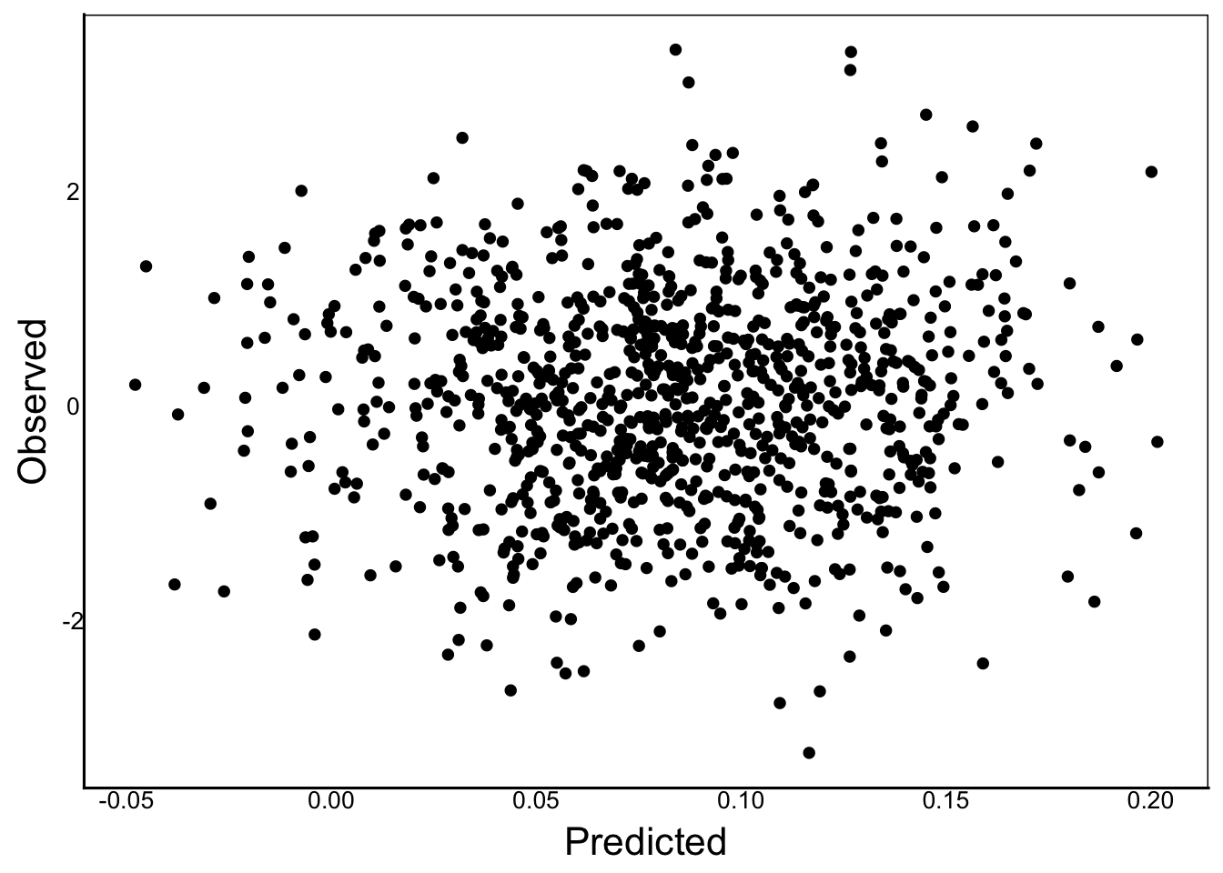

Yup, garbage, as expected.

ggplot() +
  geom_point(aes(x=predict(ComplexMod),y=InDat$Total)) +
  xlab("Predicted") + ylab("Observed")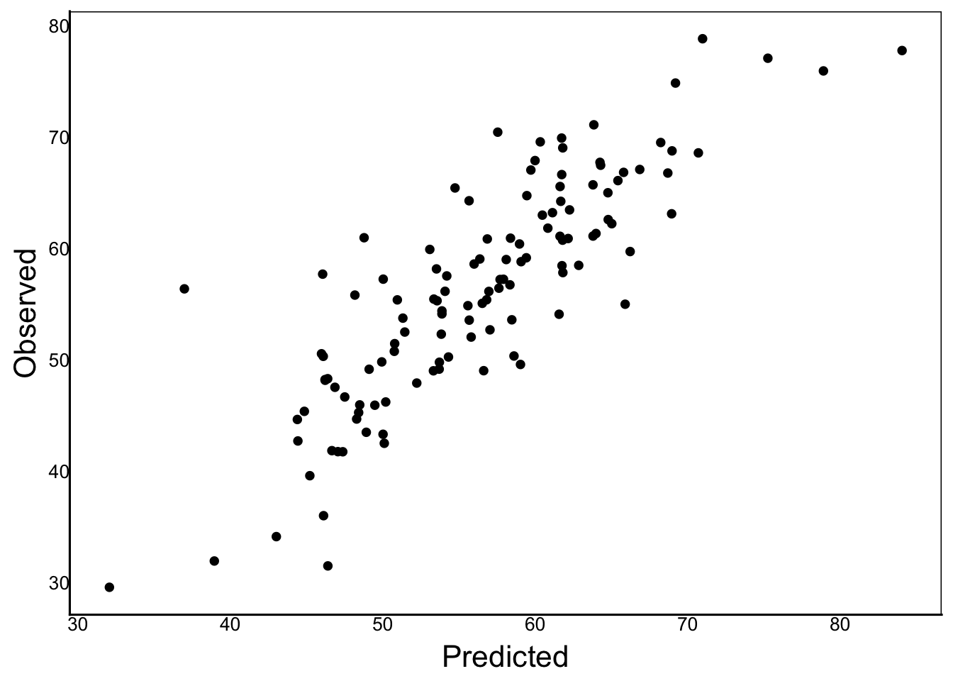

Much better!