Preface
A Crash Course in R Statistics for Biologists
Preface
This book is a companion to the R Crash Course for Biologists book. If you aren’t already familiar with R, you should start there. Links to the latest versions are available on the Colautti Lab Website: https://EcoEvoGeno.org including a free version (pdf and e-book). Print and proprietary versions (e.g. Kindle, Kobo, Apple, Google) are also available for purchase. My salary is covered by Queen’s University, so proceeds from these sales directly support students to help develop new content, including translations, online content, teaching tools, and content for future book chapters. Your support is greatly appreciated, and please don’t hesitate to reach out at the email available on our lab website.
The R Crash Course for Biologists covers the fundamentals of the R Programming language, focusing on applications for data management and visualizations. Many of the same suggestions in that book apply here, including the need to learn by doing – type out every single line of code. Making the extra effort to type everything out and compare the code and results with the book is the most efficient way to learn when you are starting out.
To get the most out of this book, R Stats Crash Course for Biologists, you should be comfortable visualizing and managing data in the R programming language. Once you have established a foundation in the R programming language, this book focuses on understanding prediction and inference from statistical models for the analysis of biological data.
This book is offered to you at a minimal cost in the hope that you will provide feedback to the author including errors, mistakes, and any supportive comments of constructive criticism that you are willing to provide.
Why R Stats?
The modern age is a ‘golden age’ for biology. Rapid developments in biochemistry, computer science, and communications have combined to revolutionize broad field of biology. It doesn’t matter if you are interested in global patterns of biodiversity or the inner complexities of a living cell, most biological questions today are addressed with data.
You may be interested in observational data sets or you may be focused on finely-controlled experiments. In either case, there are a few times where the data may ‘speak for themselves’. For example, it might be enough to show a graph of average global temperatures, or a picture of a plant or animal containing a knockout mutation with a large effect on phenotype. But what if you are looking at temperatures in different locations, or if your gene has a smaller effect on phenotype that changes with different growing conditions or genetic backgrounds? In cases like these, graphs produced with the ggplot can help to detect more subtle patterns, but it’s often not enough to have a high degree of certainty.
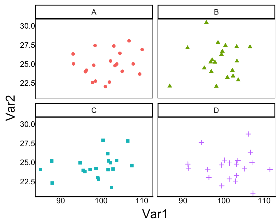
For example, look at the four-panel graph below and see which patterns stand out for you with the four variables:
Question: Which patterns are evident in these graphs?
Do you see it? Look again. Here is the reproducible code for the above graph:
set.seed(42)
PDat<-data.frame(Group=rep(c("A","B","C","D"),80),
                 Var1=rnorm(80,mean=100,sd=5),
                 Var2=rnorm(80,mean=25,sd=2))
ggplot(aes(x=Var1,y=Var2,colour=Group,shape=Group),
       data=PDat)+geom_point()+facet_wrap(vars(Group))
As you can see, these graphs were produced by random sampling. If you finished the R Crash Course for Biologists or you have a similar background coding in R, then you should understand this code. If not, you may want to review that book, particularly the R Fundamentals Chapter and the Visualizations Chapters.
So, what do those four graphs show? Nothing in particular. It turns out that the human brain is very good at ‘detecting’ patterns that aren’t really there. Patterns that look like they contain biologically meaningful results can just be random noise. Luckily, we have statistical models to keep our faulty intuitions in check.
The goal of this book is to give you a toolkit that you can use to analyze and interpret biological patterns in data, regardless of the source. We will focus heavily on simulations to apply conceptual models to understand how to identify statistical patterns and interpret their cause. Statistics generally come in two main ‘flavours’: Frequentist and Bayesian.
Frequentist vs Bayesian
One of the epic battles in modern statistics is the ongoing disagreement between two philosophies in statistics, often called the Frequentists and the Bayesians. Like most epic battles in science, this one persists because neither is superior, with inherent benefits and shortfalls in each approach and adherents to one side or the other failing to consider the merits of the alternatives.
Frequentist models have a long history in Biology, including the analysis of Francis Galton in the 1880s, Karl Pearson in the 1920s, and Ronald A Fisher in the 1940s, who were interested in continuously distributed traits. Modern frequentist statistics owes to the influence of R. A. Fisher from 1918 into the 1930s, including the development of contingency tables, and the F-statistics for the Analysis of Variance (ANOVA), with analogues that he applied to population genetics (e.g. \(F_{ST}\)). We’ll cover some of these and other frequentist models in this book. We’ll also touch on the racist origin of these methods and the persistent myth of genetic races.
Bayesian statistics is named after Thomas Bayes who developed these methods in the 1760s. As you can see by comparing years, Bayesian statistics has a longer history in mathematics, but applications in biology are much more recent than frequentist models because of its reliance on computation and iteration that were not available until more recently. Some key foundations of Bayesian statistics are introduced in this book, namely the information criteria and Fishers’ maximum likelihood estimator used in model selection. However, we focus primarily on frequentist statistics as a basis for understading the key concepts of statistical models that are shared between frequentist and Bayesian approaches. By the time you complete this book, you will have a strong understanding of frequentist models and a firm basis for exploring Bayesian statistics. If you decide to go down the Bayseian rabbit hole, I strongly recommend Statistical Rethinking by Richard McElreath (CRC Press).
Setup
Be sure to follow these steps to set up R and R Studio. You can skip this if you have already set these up from the R Crash Course book.
R
Before you begin these tutorials, you should install the latest version of R: https://cran.r-project.org/
Versions are available for Windows, MacOS and Linux operating systems. Just as we saw with base R in the R Crash Course for Biologists, a major advantage of running statistical models in R is that we can move code across computing platforms quite easily, as long as R is installed there. We can also combine our statistical models with a fully reproducible data wrangling and visualization in a professional R Markdown report! This allows for a completely reproducible analysis that will be the envy of your peers.
R Studio
You should also install R Studio: https://rstudio.com/products/rstudio/download/#download
You should be quite familiar with R and R Studio by now, but here is a quick refresher. R Studio is an Integrated Development Environment (IDE). Once you install R Studio, go ahead and run the program. You will see several helpful tabs, probably arranged across four windows. Several windows have more than one tab at the top, which you can click to access. Here is a quick overview of the more useful ones you should be familiar with.
- Environment keeps track of all of the objects in your programming environment. If this doesn’t make sense now, it will later.
- History keeps track of the code you have run.
- Files similar to the Finder (MacOS) or File Explorer (Windows), starting with the working directory.
- Plots are where your plots are created.
- Packages show which packages you have installed, and which have been loaded.
- Help provides documentation for R functions.
- Console the interface with the R program.
R Script
In R Studio you can click File-->New File-->R Script. This will open a new tab window called Untitled. This is a text file, with a .R suffix, that you can use to keep track of your R program. These are sent to the R Console to run.
Packages
Once again, we will rely on functions from tidyverse. If you aren’t already familiar, the tidyverse package contains many useful functions for working with different types of data, including visualizations with ggplot2 and data wrangling with dplyr. You’ll need to make sure you are connected to the internet and that your connection to the internet won’t be interrupted during the download.
install.packages("tidyverse")Most of the statistical models we will use are part of the stats package, which is installed and loaded automatically when you start R. In addition to the stats packages there are a few more advanced packages that we’ll explore. You may want to install them now, or wait until the appropriate chapter.
The MuMIn and MASS packages in R have some convenient functions for running model selection. lmtest is used for a particular type of model selection called the Likelihood Ratio Test. We’ll look at Mixed Effects models, using the lme4 package. Finally, we’ll use the mgcv library for Generalized Additive Models (GAM) and Generalized Additive Mixed Models (GAMM).