Generalized Additive Models

Introduction

You should now be familiar with Linear Models (LM), Generalized Linear Models (GLM) and Generalized Linear Mixed Effects (GLME) models.

Be sure to review and understand the similarities and differences so that you understand how GLM, LME, and GLME expand on LM by incorporating other forms of estimates and error variances. In this tutorial we add another tool to the statistical toolbox. Generalized Additive Models (GAM) are an extension of polynomial regression but allowing more complex curves and interactions.

A general function for a GAM is:

\[g(Y) = \beta_0 + s_1(X_1) + ... + s_k(X_k) + \epsilon\]

The terms g() and s() denote functions or transformations of the data. The g() term we have seen before, this is the link function just like we saw with the Generalized Linear Models (GLM). The link function just transforms the variable based on its error distribution (e.g. binomial, Poisson, Gaussian). The s() functions are smoothing functions that expand from linear models with a single slope to include more complex functions.

The smoothing functions are estimated directly from the data, rather than fitting slopes like we do with standard linear regression. This involves some complex math that you won’t need to know to apply and interpret GAM results, so we won’t examine it here. Just remember that s() is some kind of function. The complexity of the smoothing function is given by a parameter \(\lambda\).

\(\lambda\) is a parameter that is commonly used in machine learning models. For now, just know that \(\lambda\) is a parameter that acts as a penalty for over-fitting the data. A higher \(\lambda\) value produces a smoother (i.e. less wiggly) curve.

Setup

We’ll be using the mgcv library for Generalized Additive Models (GAM) and Generalized Additive Mixed Models (GAMM):

library(mgcv)

Loading required package: nlme

This is mgcv 1.9-4. For overview type '?mgcv'.

The usual setup for plotting, data management, and likelihood ratio test (for model selection)

library(ggplot2) # plotting library

Warning: package 'ggplot2' was built under R version 4.5.2

library(dplyr) # data management

Attaching package: 'dplyr'

The following object is masked from 'package:nlme':

    collapse

The following objects are masked from 'package:stats':

    filter, lag

The following objects are masked from 'package:base':

    intersect, setdiff, setequal, union

library(lmtest)

Loading required package: zoo

Warning: package 'zoo' was built under R version 4.5.2

Attaching package: 'zoo'

The following objects are masked from 'package:base':

    as.Date, as.Date.numeric

# Set custom plotting theme
source("http://bit.ly/theme_pub") 
theme_set(theme_pub())

Import data from the 2013 Science Paper “Rapid adaptation to climate facilitates range expansion of an invasive plant”: https://doi.org/10.1126/science.1242121

LythrumDat<-
  read.csv("https://colauttilab.github.io/Data/ColauttiBarrett2013Data.csv",
           header=T)

Data Overview

This data is from a published paper, and it’s available for free from the Dryad repository: https://doi.org/10.5061/dryad.878m3

The Dryad Repository (datadryad.org) is a great place to find data sets to practice your analytic skills or to explore new ideas.

Like most data in the repository, the dataset we will be working on is a bit more complicated than most of the examples we’ve simulated in the other chapters. So we’ll take some time to understand the data before moving on. Full detail is available in the Science paper “Colautti & Barrett (2013)”: https://doi.org/10.1126/science.1242121

But here we’ll focus on a few aspects of the data. The main question we’ll look at today is:

How does natural selection act on Flowering time?

The paper reports on a reciprocal transplant experiment. This is a classic experimental design in which genotypes are collected from different geographic locations, and reared together in different environments.

In this case, seeds were collected from different maternal ‘families’ along a latitudinal gradient, and then grown at 3 locations along the same gradient. This is a common approach for natural populations. Since two individuals from the same maternal family share somewhere between 1/4 (half-sibling) to 1/2 (full-sibling) of their genes in common, we can use statistical methods to estimate how much a particular phenotype depends on individuals sharing the same genes. We call this the ‘genetic effect’ on phenotype.

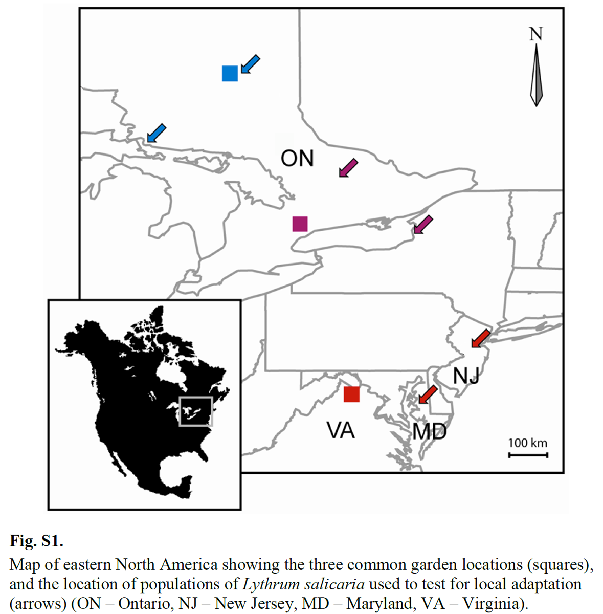
In this experiment, there were 4 growing seasons from 2007 to 2010. Traits measured in each year are Julian Day of first flower, height of the vegetative portion of the plant, inflorescence biomass, and number of fruits. Seed families were sampled from six locations and the entire experiment was replicated at three geographic locations along a latitudinal gradient: Timmons (ON), Newmarket (ON) and northern Virginia.

This map from the Supplementary Material of the paper shows the locations of the seed collections (arrows) and common garden locations (squares).

Looking at the structure of the data:

str(LythrumDat)

• Ind – A unique identifier for each plant in the experiment
• Site – The common garden location: BEF = South, KSR = Mid, Timmins = North
• Row & Pos – location within the common garden
• Mat – A unique identifier for each maternal family
• Pop – The Population (seed location) in alphabetical order from North (A) to South (T)
• Region – The geographical region of the saampled population. There are 3 regions (North, Mid, South) with two populations from each region
• Flwr – Julian Day of first flower
• FVeg – Height of the vegetative part of the plant, measured on the day that the plant started to flower
• HVeg – Height of the vegetative part of the plant, measured at the end (post-harvest)
• InfMass – Mass of the inflorescence, which previous studies show is a good estimate of total seeds production
• Fruits07 – Number of fruits measured in 2007; can be used to test relationship between fruit number and inflorescence biomass.

Where in the list above denotes a 2-digit number that refers to year of collection from 2007 (07) through 2010 (10).

Fitness

Fitness in this experiment is measured as lifetime reproduction over the four growing seasons. For this we can simply sum the InfMass<XX> columns, but first we should replace NA with 0, since missing biomass in this data set represents a plant that produces no offspring.

SelDat<-LythrumDat %>%
  mutate(InfMass07 = ifelse(is.na(InfMass07),0,InfMass07),
         InfMass08 = ifelse(is.na(InfMass08),0,InfMass08),
         InfMass09 = ifelse(is.na(InfMass09),0,InfMass09),
         InfMass10 = ifelse(is.na(InfMass10),0,InfMass10)
         ) %>%
  mutate(Fitness = InfMass07 + InfMass08 + InfMass09 + InfMass10)

Now we can try to visualize the distribution of fitness. We should probably look at each site separately

ggplot(aes(x=Fitness), data=SelDat) + geom_histogram(bins=20) +
  facet_wrap("Site",ncol=1)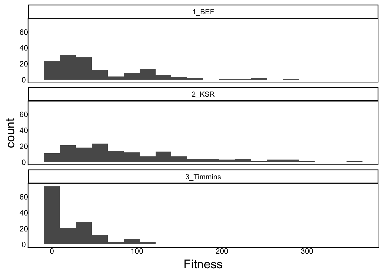

Phenotypes

The main traits under selection in this experiment are flowering time and vegetative size. These are measured in each year, so we can see how consistent they are across growing seasons.

ggplot(aes(x=Flwr08, y=Flwr09), data=SelDat)+geom_point()

Warning: Removed 106 rows containing missing values or values outside the scale range
(`geom_point()`).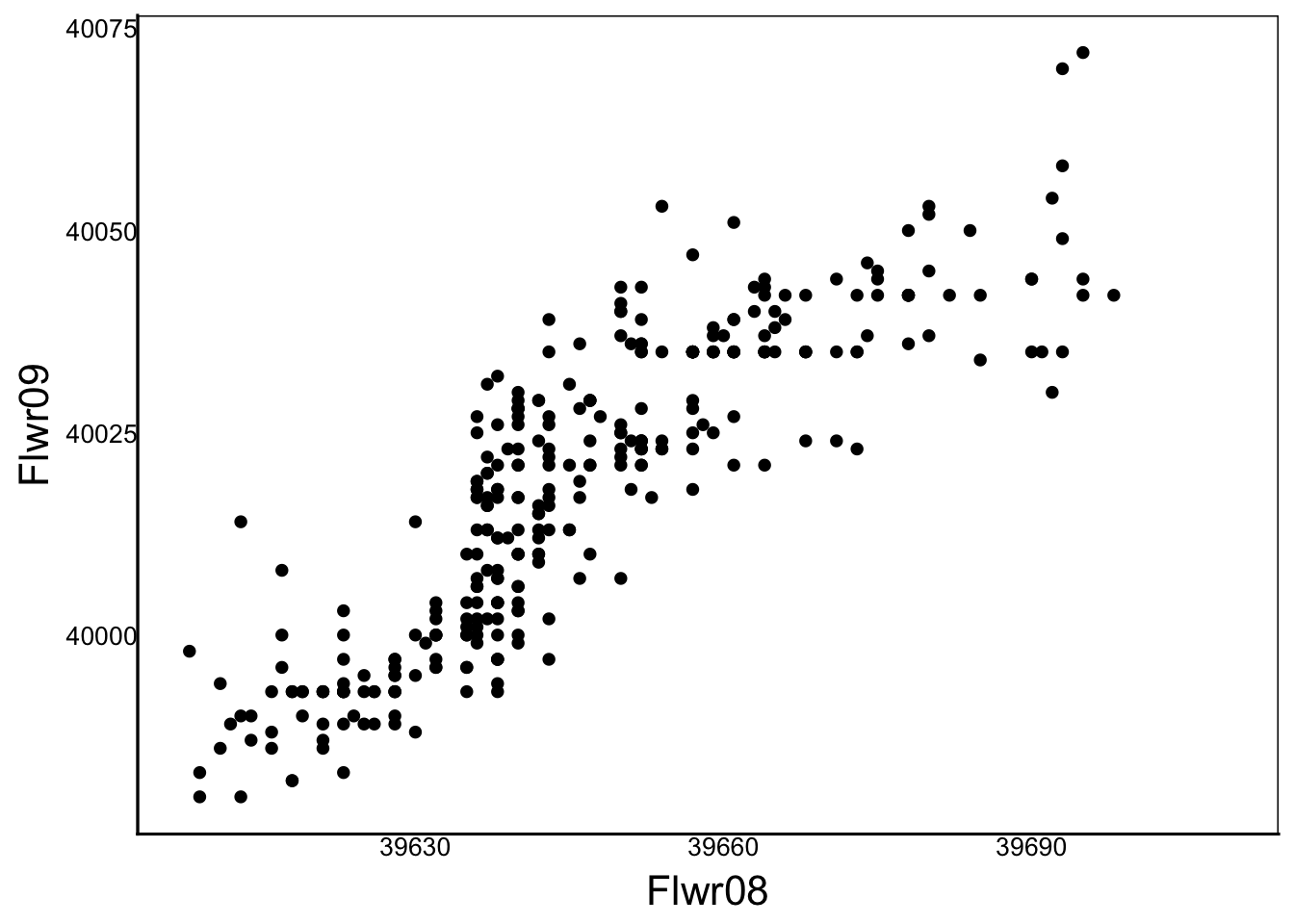

Because they are correlated, we will make the analysis easier by averaging the flowering time and size across years.

Before we can do this, we have to adjust the Flwr<XX> columns because the values here include the year of measurement. You can see this by comparing the values on the x vs y-axis and you can see that the values of y are advanced by about 365 days.

To standardize day within year, we’ll take a shortcut, and just adjust each to the earliest value within each year.

SelDat<-SelDat %>%
  mutate(Flwr07 = Flwr07 - min(Flwr07,na.rm=T),
         Flwr08 = Flwr08 - min(Flwr08,na.rm=T),
         Flwr09 = Flwr09 - min(Flwr09,na.rm=T),
         Flwr10 = Flwr10 - min(Flwr10,na.rm=T))

Now we can calculate the average day across years:

SelDat<-SelDat %>% rowwise() %>%
  mutate(FlwrAvg = mean(c(Flwr07,Flwr08,Flwr09,Flwr10), na.rm=T),
         FVegAvg = mean(c(FVeg07,FVeg08,FVeg09,FVeg10), na.rm=T),
         )

Note we use the rowwise() function here with mutate to average across rows, instead of the usual averaging down columns

Next, we should also look at these distributions to make sure we did the calculations properly and we don’t have any outlier data.

ggplot(aes(x=FlwrAvg), data=SelDat) + geom_histogram(bins=20) + 
  facet_wrap("Site",ncol=1)

Warning: Removed 49 rows containing non-finite outside the scale range
(`stat_bin()`).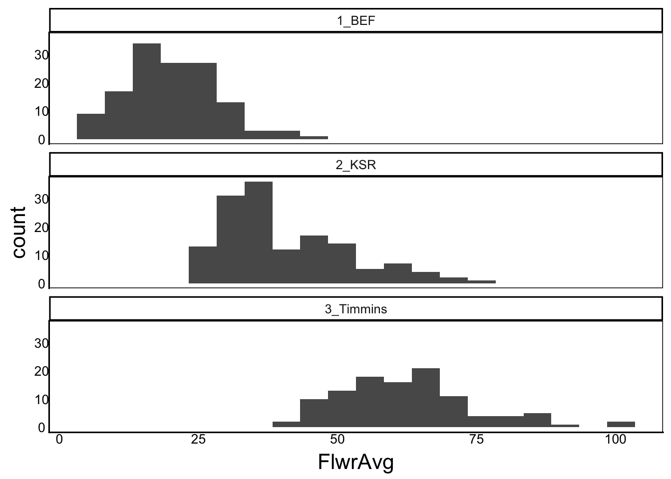

ggplot(aes(x=FVegAvg), data=SelDat) + geom_histogram(bins=20) + 
  facet_wrap("Site",ncol=1)

Warning: Removed 49 rows containing non-finite outside the scale range
(`stat_bin()`).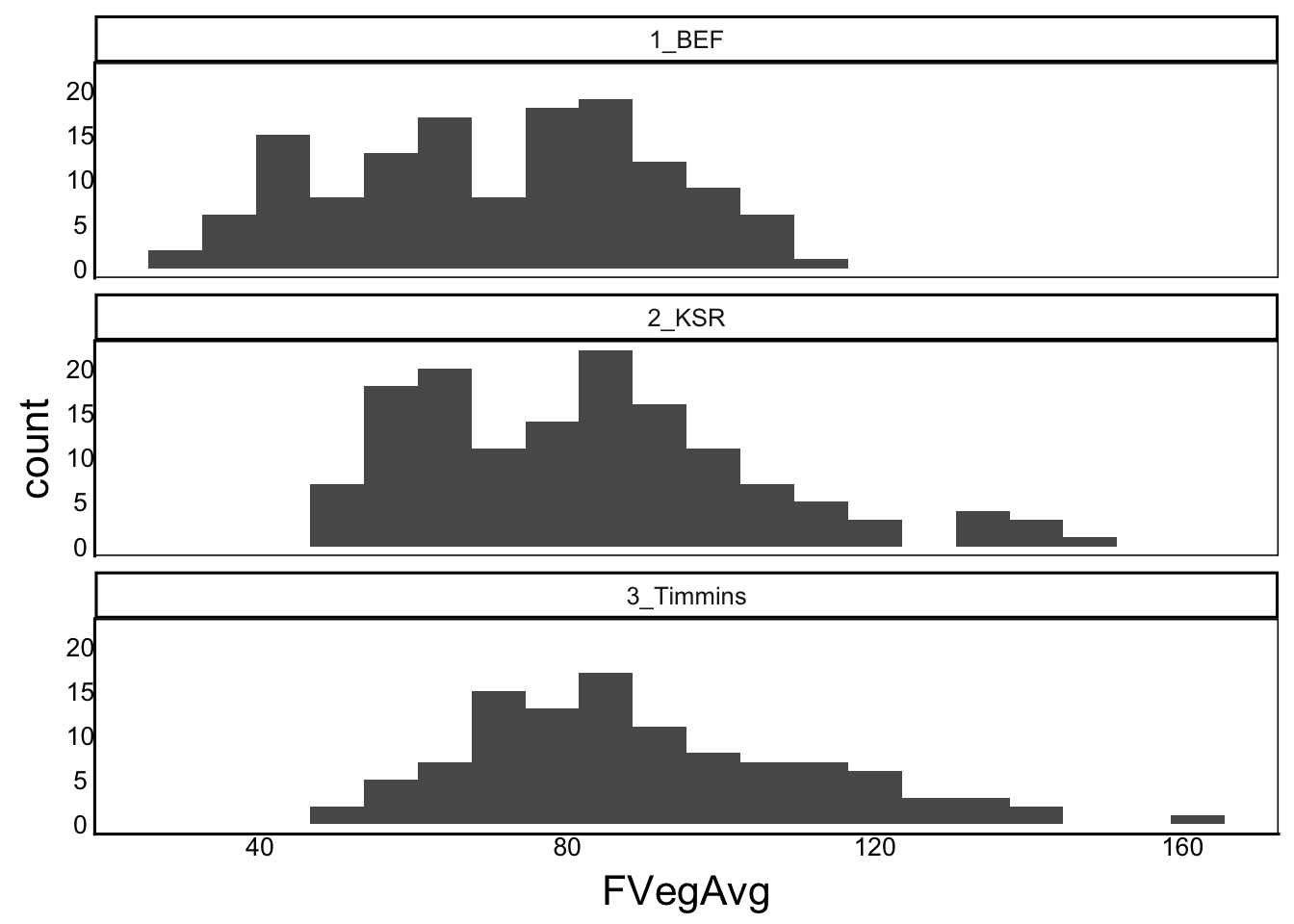

Measuring Phenotypic Selection

Natural selection is a core concept in evolutionary biology, which we can actually measure statistically. Specifically, we can measure natural selection acting on any phenotypic trait by looking at its linear and non-liner relationship with fitness. In practice, we often can’t measure fitness directly, but we can get close by measuring survival and reproduction. This is done through a multiple regression, with a significant linear estimate representing directional selection favouring larger trait values if the slope is positive and smaller trait values if the slope is negative. We can also test for stabilizing selection on a trait as a nonlinear relationship representing either stabilizing selection that favours intermediate traits values or disruptive selection that favours extreme values.

Four types of phenotypic selection inferred from linear and quadratic regression

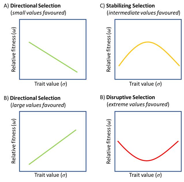
In summary, we are generally interested in two phenomena in phenotypic selection analysis:

1. Directional Selection – This is just the linear relationship between a trait and fitness and may be used to predict evolution in response to selection. Evolution is predicted to increase (or decrease) the population trait mean if the slope of the regression is positive (or negative).
2. Stabilizing/Disruptive Selection – This is typically a quadratic regression with thepoly(x,2) function. It tests whether selection favours an optimum phenotype (stabilizing selection) if the coefficient estimate is negative or extreme phenotypes (disruptive selection) if the coefficient estimate is positive.

Typically, we should standardize both the phenotypic traits and fitness. Each of our phenotypic traits can be transformed to a \(z\)-scores (\(mean = 0\) and \(sd = 1\)), as described in the Distributions Chapter. In contrast, fitness is usually transformed by dividing each value by the overall mean (\(x_i/\bar x\)) – this is known as **relative fitness*, which is often denoted using the lower-case ‘omega’ character (\(\omega\)).

Any statistical function fit to these data can be compared across studies, regardless of traits, organisms, or fitness measurements. The fitness function predicts multiples of fitness as a function of trait standard deviations. For example, a linear slope of -2 means that increasing the trait by one standard deviation reduces fitness by a multiple of 2.

Relative Fitness

SelDat$Fitness<-SelDat$Fitness/mean(SelDat$Fitness)

Standardize Traits

Before we standardize our traits, we must be careful to think about our missing data. In the case of fitness, we assumed NA = 0 because a plant either died or produced no viable seeds, which is a zero for fitness. But we also have NA values for flowering time and vegetative size. In these cases, the plant may have died early in the experiment before reaching maturity, so we have no way of knowing what the phenotype would have been if they survived. These should be removed from our analysis:

SelDat<-SelDat %>%
  filter(!is.na(FlwrAvg) &
         !is.na(FVegAvg))

Now that we have removed missing values, we standardize to \(z\)-scores:

SelDat$FlwrAvg<-(SelDat$FlwrAvg-
                   mean(SelDat$FlwrAvg))/sd(SelDat$FlwrAvg)
SelDat$FVegAvg<-(SelDat$FVegAvg-
                   mean(SelDat$FVegAvg))/sd(SelDat$FVegAvg)

\(s\) vs \(\beta\)

We can estimate phenotypic selection in two ways. We can model each trait individually – the linear regression estimate from this model is known as the selection differential (\(s\)). Alternatively, we can include all traits in a single statistical model – the individual regression estimates for each trait in this model are known as the selection gradients (\(\beta\)). In the Advanced Linear Models tutorial, we saw that the partial coefficients from the combined model may be quite different from the regular coefficients of the individual statistical models, depending on how the different predictors are correlated. Likewise, the selection differential (\(s\)) is an estimate of how a population will respond to selection, whereas the selection gradient (\(\beta\)) is an estimate of how a population would respond to selection if it wasn’t constrained by selection acting on correlated traits.

Linear Models

Now that our traits are transformed, we are ready for the analysis. Later we will see how to use GAMs to look at more complicated fitness functions, but for now let’s review how we might analyze this using linear models.

We might predict that selection on flowering time will be stronger in the north compared to the south, because of the shorter growing season. We also might predict that larger plants are favoured everywhere.

Selection Differentials

We can run a simple linear regression model with separate slopes for each Site. Later, we will include both traits in a single multiple regression. we analyze each trait in a separate model

LRModF<-lm(Fitness ~ FlwrAvg*Site, data=SelDat)
summary(LRModF)

Call:
lm(formula = Fitness ~ FlwrAvg * Site, data = SelDat)

Residuals:
    Min      1Q  Median      3Q     Max 
-1.7387 -0.6358 -0.2330  0.4127  4.6455 

Coefficients:
                      Estimate Std. Error t value Pr(>|t|)    
(Intercept)             1.4754     0.2290   6.443 3.58e-10 ***
FlwrAvg                 0.4717     0.2161   2.183  0.02966 *  
Site2_KSR               0.1983     0.2445   0.811  0.41785    
Site3_Timmins          -0.4480     0.3111  -1.440  0.15075    
FlwrAvg:Site2_KSR      -0.4166     0.2629  -1.585  0.11383    
FlwrAvg:Site3_Timmins  -0.8882     0.2690  -3.302  0.00105 ** 
---
Signif. codes:  0 '***' 0.001 '**' 0.01 '*' 0.05 '.' 0.1 ' ' 1

Residual standard error: 1.017 on 377 degrees of freedom
Multiple R-squared:  0.1928,    Adjusted R-squared:  0.182 
F-statistic:    18 on 5 and 377 DF,  p-value: 5.08e-16

We see that the slope in the southern site (FlwrAvg) is positive, but by adding estimates to calculate slopes in other regions, we can see it is close to zero at the mid-latitude site (FlwrAvg + FlwrAvg:Site2_KSR), with a strongly negative slope in the northern site (FlwrAvg + FlwrAvg:Site3_Timmins). These are the site-specific selection differentials (\(s\)). We can also visualize this by graphing:

ggplot(aes(x=FlwrAvg, y=Fitness), data=SelDat) + geom_point() + 
  facet_wrap("Site",ncol=1) + geom_smooth(method="lm")

`geom_smooth()` using formula = 'y ~ x'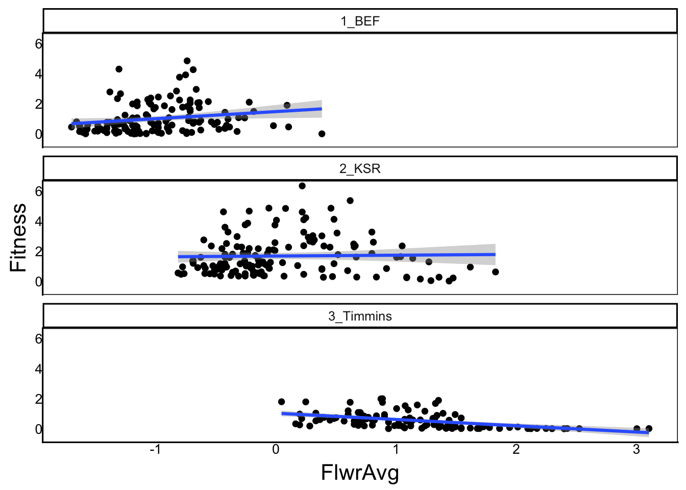

We can do the same for vegetative size:

LRModV<-lm(Fitness ~ FVegAvg*Site, data=SelDat)
summary(LRModV)

Call:
lm(formula = Fitness ~ FVegAvg * Site, data = SelDat)

Residuals:
    Min      1Q  Median      3Q     Max 
-2.5164 -0.5105 -0.1618  0.3404  4.3411 

Coefficients:
                      Estimate Std. Error t value Pr(>|t|)    
(Intercept)            1.30945    0.08996  14.557  < 2e-16 ***
FVegAvg                0.69085    0.09200   7.509 4.35e-13 ***
Site2_KSR              0.32930    0.11968   2.752  0.00622 ** 
Site3_Timmins         -0.73294    0.13330  -5.499 7.07e-08 ***
FVegAvg:Site2_KSR     -0.29116    0.12239  -2.379  0.01785 *  
FVegAvg:Site3_Timmins -0.77237    0.13127  -5.884 8.86e-09 ***
---
Signif. codes:  0 '***' 0.001 '**' 0.01 '*' 0.05 '.' 0.1 ' ' 1

Residual standard error: 0.9363 on 377 degrees of freedom
Multiple R-squared:  0.316, Adjusted R-squared:  0.3069 
F-statistic: 34.83 on 5 and 377 DF,  p-value: < 2.2e-16

Again we get a shift from positive to negative slope going from the southern garden (1_BEF) to then northern garden (3_Timmins).

ggplot(aes(x=FVegAvg, y=Fitness), data=SelDat) + geom_point() + 
  facet_wrap("Site",ncol=1) + geom_smooth(method="lm")

`geom_smooth()` using formula = 'y ~ x'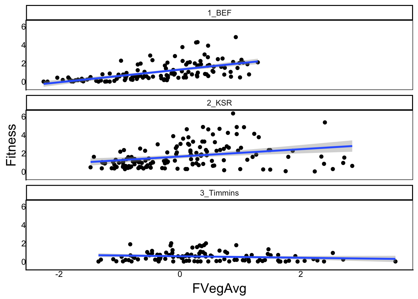

By analyzing these as separate models, we assume the traits are independent. In fact, they are correlated:

ggplot(aes(x=FlwrAvg, y=FVegAvg), data=SelDat) + geom_point()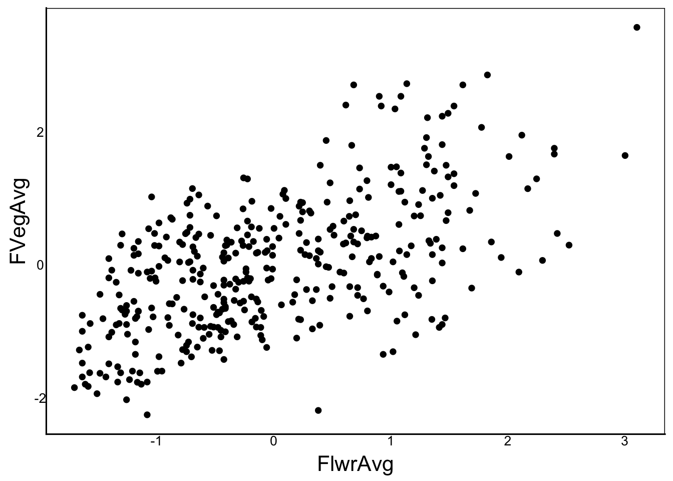

cor(SelDat$FlwrAvg,SelDat$FVegAvg)

[1] 0.5906049

Plants that delay flowering generally get bigger than plants that flower early. This means that observations for one of these traits is not independent of the other, and therefore we shouldn’t analyze them in separate models. Since the correlation is not too strong, we can solve the problem by including both as predictors in the model.

Question: What would happen if these traits were highly correlated and we included them both as predictors?

Answer: Review collinearity in the Advanced Linear Models chapter if you don’t remember.

Multiple Regression

As noted earlier, we can include both traits in a multiple regression to estimate selection gradients (\(\beta\)).

MRMod<-lm(Fitness ~ FlwrAvg*Site + FVegAvg*Site, data=SelDat)
summary(MRMod)

Call:
lm(formula = Fitness ~ FlwrAvg * Site + FVegAvg * Site, data = SelDat)

Residuals:
    Min      1Q  Median      3Q     Max 
-2.5247 -0.5207 -0.1404  0.2977  4.0640 

Coefficients:
                       Estimate Std. Error t value Pr(>|t|)    
(Intercept)            0.908264   0.210616   4.312 2.07e-05 ***
FlwrAvg               -0.459690   0.221082  -2.079  0.03827 *  
Site2_KSR              0.734714   0.223273   3.291  0.00109 ** 
Site3_Timmins          0.139189   0.281403   0.495  0.62115    
FVegAvg                0.804677   0.102259   7.869 3.89e-14 ***
FlwrAvg:Site2_KSR     -0.931927   0.310018  -3.006  0.00283 ** 
FlwrAvg:Site3_Timmins  0.008938   0.270132   0.033  0.97362    
Site2_KSR:FVegAvg      0.249657   0.163251   1.529  0.12704    
Site3_Timmins:FVegAvg -0.756678   0.142035  -5.327 1.72e-07 ***
---
Signif. codes:  0 '***' 0.001 '**' 0.01 '*' 0.05 '.' 0.1 ' ' 1

Residual standard error: 0.879 on 374 degrees of freedom
Multiple R-squared:  0.4019,    Adjusted R-squared:  0.3891 
F-statistic: 31.42 on 8 and 374 DF,  p-value: < 2.2e-16

Note that we do not want the FlwrAvg:FVegAvg term yet, but we would want it for a quadratic model testing for stabilizing or disruptive selection. Compare these coefficients (\(\beta\)) with the above (\(s\)). For example, FlwrAvg has switched from positive to negative. We can also test the fit of the model using model selection. Since the simpler model is Flowering time OR vegetative size, we should compare both.

lrtest(LRModF,MRMod)

Likelihood ratio test

Model 1: Fitness ~ FlwrAvg * Site
Model 2: Fitness ~ FlwrAvg * Site + FVegAvg * Site
  #Df  LogLik Df  Chisq Pr(>Chisq)    
1   7 -546.92                         
2  10 -489.49  3 114.87  < 2.2e-16 ***
---
Signif. codes:  0 '***' 0.001 '**' 0.01 '*' 0.05 '.' 0.1 ' ' 1

lrtest(LRModV,MRMod)

Likelihood ratio test

Model 1: Fitness ~ FVegAvg * Site
Model 2: Fitness ~ FlwrAvg * Site + FVegAvg * Site
  #Df  LogLik Df  Chisq Pr(>Chisq)    
1   7 -515.21                         
2  10 -489.49  3 51.436  3.949e-11 ***
---
Signif. codes:  0 '***' 0.001 '**' 0.01 '*' 0.05 '.' 0.1 ' ' 1

We can also do a LRT to figure out if we need the three-way interaction and all of the two-way interactions.

Challenge: Test each of the 2-way interaction terms in MRMod model using LRT

Review the Model Selection chapter if you aren’t sure how to do this. Take the time to do this. If you have trouble, then you don’t know model selection as well as you think you do!

QC Problem

Now let’s take a look at our model assumptions:

ggplot()+
  geom_point(aes(x=predict(MRMod),y=residuals(MRMod)))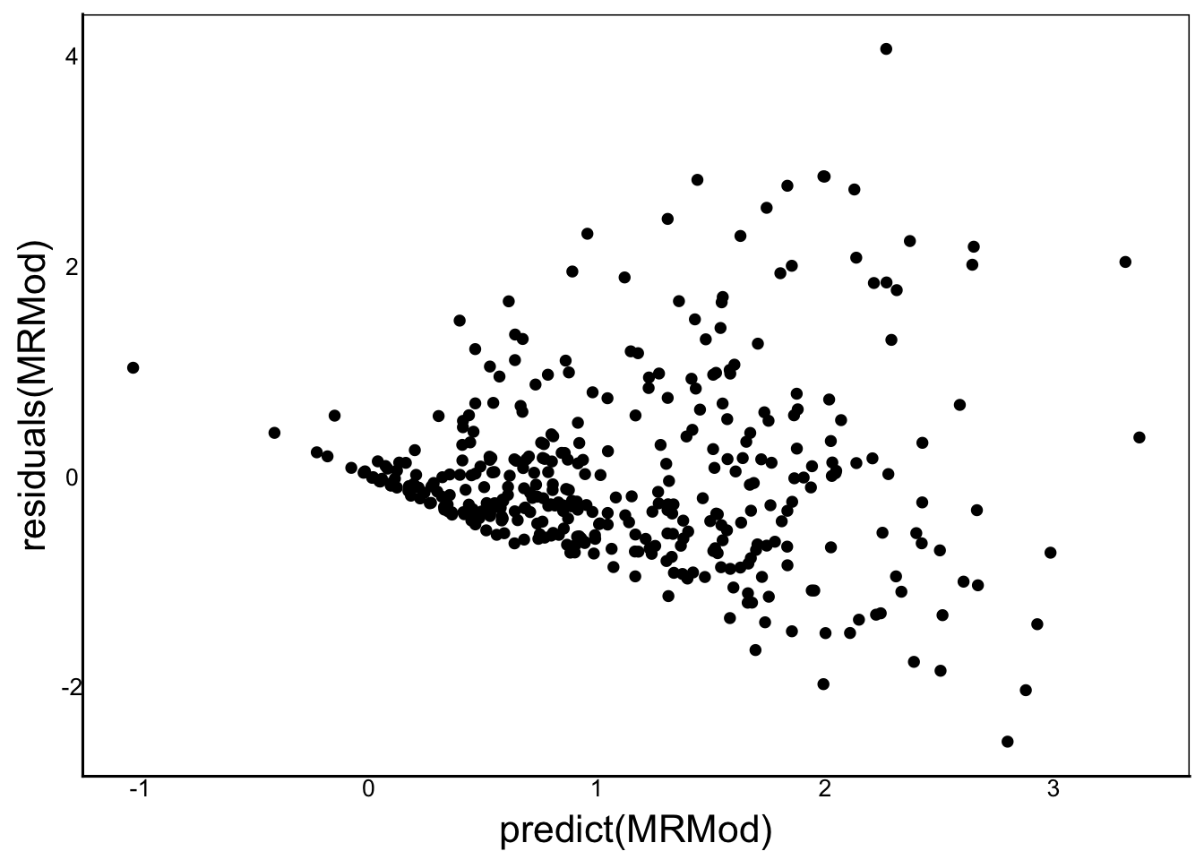

There is clearly a big problem with the assumption of homogeneous variance. Looking back at the graphs of fitness vs FlwrAvg and FVegAvg we can see that there may be some non-linearity in the relationships. In fact, our measure of fitness is inflorescence biomass, which correlates with fruit or seed number – both count data likely to follow a Poisson distribution. We’ll come back to this point later when we run a GAM.

Polynomial Regression

In the Linear Models Chapter we saw how polynomial regression was a special case of a linear model.

In Polynomial regression, we want add different powers of the same predictor:

\[ Y \sim \beta_0 + \beta_1X_1 + \beta_2X_{1}^{2} + \beta_3X_{1}^{3} + ...\]

Technically, we should zero-center each predictor (\(X_k\)) before raising it to a power, otherwise we will have collinear predictors. The poly() function provides a convenient way to implement this quickly in R.

In this data set, we should separate parameters for each common garden location, which means we want three slopes for each \(\beta\) slope in the model above.
For a selection analysis we would typically be interested in only the linear and quadratic terms, which would test for directional selection (linear) and for stabilizing or disruptive selection (squared term). However, we can also test for more complicated fitness relationships using model selection.

QuadModF<-lm(Fitness ~ poly(FlwrAvg,degree=2)*Site, data=SelDat)

Does the quadratic model fit better than the simpler linear model?

lrtest(QuadModF,LRModF)

Likelihood ratio test

Model 1: Fitness ~ poly(FlwrAvg, degree = 2) * Site
Model 2: Fitness ~ FlwrAvg * Site
  #Df  LogLik Df  Chisq Pr(>Chisq)    
1  10 -524.67                         
2   7 -546.92 -3 44.511  1.175e-09 ***
---
Signif. codes:  0 '***' 0.001 '**' 0.01 '*' 0.05 '.' 0.1 ' ' 1

Yes, it’s a highly significant difference, so the quadratic model fits the data much better. This shows that there is curvature to the relationship. We can look at the summary and plot to better understand how:

summary(QuadModF)

Call:
lm(formula = Fitness ~ poly(FlwrAvg, degree = 2) * Site, data = SelDat)

Residuals:
    Min      1Q  Median      3Q     Max 
-1.9335 -0.5631 -0.1574  0.3637  4.1475 

Coefficients:
                                         Estimate Std. Error t value Pr(>|t|)
(Intercept)                               -0.2048     0.6056  -0.338  0.73548
poly(FlwrAvg, degree = 2)1               -36.5404    15.9113  -2.297  0.02220
poly(FlwrAvg, degree = 2)2               -24.0016     8.0777  -2.971  0.00316
Site2_KSR                                  0.9767     0.6287   1.554  0.12112
Site3_Timmins                              1.1949     0.7684   1.555  0.12076
poly(FlwrAvg, degree = 2)1:Site2_KSR      42.0428    16.1674   2.600  0.00968
poly(FlwrAvg, degree = 2)2:Site2_KSR      -4.6859     9.3455  -0.501  0.61638
poly(FlwrAvg, degree = 2)1:Site3_Timmins  29.0777    17.9703   1.618  0.10649
poly(FlwrAvg, degree = 2)2:Site3_Timmins  23.6669     8.9481   2.645  0.00852
                                           
(Intercept)                                
poly(FlwrAvg, degree = 2)1               * 
poly(FlwrAvg, degree = 2)2               **
Site2_KSR                                  
Site3_Timmins                              
poly(FlwrAvg, degree = 2)1:Site2_KSR     **
poly(FlwrAvg, degree = 2)2:Site2_KSR       
poly(FlwrAvg, degree = 2)1:Site3_Timmins   
poly(FlwrAvg, degree = 2)2:Site3_Timmins **
---
Signif. codes:  0 '***' 0.001 '**' 0.01 '*' 0.05 '.' 0.1 ' ' 1

Residual standard error: 0.9635 on 374 degrees of freedom
Multiple R-squared:  0.2813,    Adjusted R-squared:  0.266 
F-statistic:  18.3 on 8 and 374 DF,  p-value: < 2.2e-16

Recall from the Linear Models Chapter that poly(...)1 is the linear coefficient, and poly(...)2 is the quadratic (squared) coefficient.

From high-school calculus remember that the coefficient for a squared term determines whether the curve is convex or concave. A positive quadratic represents disruptive selection favouring extreme variances while a negative value represents stabilizing selection favouring intermediate values.

Note that some of these values are quite large and so are the standard errors. The high SE is a good indication that we are getting close to the limit of our data in terms of how many predictors we can include in our model.

ggplot(aes(x=FlwrAvg, y=Fitness), data=SelDat) + 
  geom_point() + 
  geom_smooth(method="lm", formula=y ~ poly(x,degree=3)) +
  facet_grid(rows=vars(Site))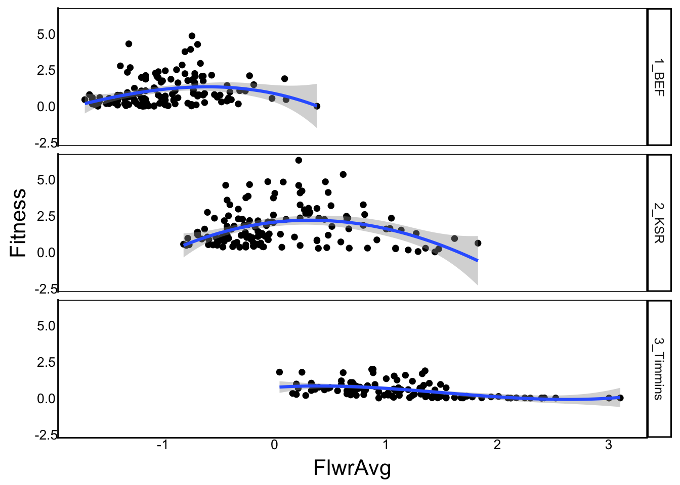

We can do the same for vegetative size:

QuadModV<-lm(Fitness ~ poly(FVegAvg,degree=2)*Site, data=SelDat)

lrtest(QuadModV,LRModV)

Likelihood ratio test

Model 1: Fitness ~ poly(FVegAvg, degree = 2) * Site
Model 2: Fitness ~ FVegAvg * Site
  #Df  LogLik Df  Chisq Pr(>Chisq)    
1  10 -495.41                         
2   7 -515.21 -3 39.597  1.297e-08 ***
---
Signif. codes:  0 '***' 0.001 '**' 0.01 '*' 0.05 '.' 0.1 ' ' 1

summary(QuadModV)

Call:
lm(formula = Fitness ~ poly(FVegAvg, degree = 2) * Site, data = SelDat)

Residuals:
    Min      1Q  Median      3Q     Max 
-2.1747 -0.4774 -0.0949  0.3214  3.9884 

Coefficients:
                                          Estimate Std. Error t value Pr(>|t|)
(Intercept)                                1.31346    0.09661  13.595  < 2e-16
poly(FVegAvg, degree = 2)1                13.74895    3.22630   4.262 2.57e-05
poly(FVegAvg, degree = 2)2                 0.25032    2.77576   0.090 0.928191
Site2_KSR                                  0.27579    0.12272   2.247 0.025206
Site3_Timmins                             -0.78545    0.13876  -5.661 3.01e-08
poly(FVegAvg, degree = 2)1:Site2_KSR      -2.37552    3.60547  -0.659 0.510388
poly(FVegAvg, degree = 2)2:Site2_KSR     -11.01983    3.27212  -3.368 0.000836
poly(FVegAvg, degree = 2)1:Site3_Timmins -13.43573    3.89766  -3.447 0.000631
poly(FVegAvg, degree = 2)2:Site3_Timmins  -3.09518    3.40217  -0.910 0.363532
                                            
(Intercept)                              ***
poly(FVegAvg, degree = 2)1               ***
poly(FVegAvg, degree = 2)2                  
Site2_KSR                                *  
Site3_Timmins                            ***
poly(FVegAvg, degree = 2)1:Site2_KSR        
poly(FVegAvg, degree = 2)2:Site2_KSR     ***
poly(FVegAvg, degree = 2)1:Site3_Timmins ***
poly(FVegAvg, degree = 2)2:Site3_Timmins    
---
Signif. codes:  0 '***' 0.001 '**' 0.01 '*' 0.05 '.' 0.1 ' ' 1

Residual standard error: 0.8927 on 374 degrees of freedom
Multiple R-squared:  0.3831,    Adjusted R-squared:   0.37 
F-statistic: 29.04 on 8 and 374 DF,  p-value: < 2.2e-16

Again, we find the quadratic is significant but this time selection is generally disruptive in the south but stabilizing in the north and intermediate at the mid-latitude site.

ggplot(aes(x=FVegAvg, y=Fitness), data=SelDat) + 
  geom_point() + 
  geom_smooth(method="lm", formula=y ~ poly(x,degree=3)) +
  facet_grid(rows=vars(Site))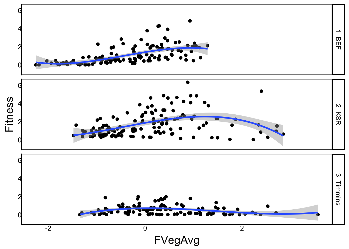

Again, these traits FVegAvg and FlwrAvg are not independent, so we should include them both in the same model. However, when we do this, we also need to think about the interaction between them. To understand why, think about the quadratic expansion of two terms:

\[ (A+B)^2 =A^2+2AB+B^2 \]

With the poly function, we get the squared terms, but not the \(2AB\) term. But we can manually add this to our model:

QuadMod<-lm(Fitness ~ poly(FlwrAvg,degree=2) * Site +
              poly(FVegAvg,degree=2) * Site + 
              FlwrAvg:FVegAvg:Site, 
            data=SelDat)
summary(QuadMod)

Call:
lm(formula = Fitness ~ poly(FlwrAvg, degree = 2) * Site + poly(FVegAvg, 
    degree = 2) * Site + FlwrAvg:FVegAvg:Site, data = SelDat)

Residuals:
    Min      1Q  Median      3Q     Max 
-2.1265 -0.4169 -0.1500  0.3095  3.5309 

Coefficients:
                                           Estimate Std. Error t value Pr(>|t|)
(Intercept)                                0.146203   0.548632   0.266 0.790014
poly(FlwrAvg, degree = 2)1               -32.707694  14.753222  -2.217 0.027240
poly(FlwrAvg, degree = 2)2                -9.324191   7.690443  -1.212 0.226129
Site2_KSR                                  0.674332   0.760564   0.887 0.375867
Site3_Timmins                              0.931649   0.727488   1.281 0.201134
poly(FVegAvg, degree = 2)1                14.012423   4.017642   3.488 0.000547
poly(FVegAvg, degree = 2)2                 5.816519   3.017258   1.928 0.054662
poly(FlwrAvg, degree = 2)1:Site2_KSR       9.667066  15.605571   0.619 0.535998
poly(FlwrAvg, degree = 2)2:Site2_KSR     -15.124777  12.985256  -1.165 0.244875
poly(FlwrAvg, degree = 2)1:Site3_Timmins  22.556051  16.890935   1.335 0.182580
poly(FlwrAvg, degree = 2)2:Site3_Timmins  10.132306   8.941086   1.133 0.257862
Site2_KSR:poly(FVegAvg, degree = 2)1       7.341296   4.785566   1.534 0.125884
Site3_Timmins:poly(FVegAvg, degree = 2)1 -11.501421   5.885833  -1.954 0.051454
Site2_KSR:poly(FVegAvg, degree = 2)2     -10.712526   5.316663  -2.015 0.044648
Site3_Timmins:poly(FVegAvg, degree = 2)2  -8.396928   3.717474  -2.259 0.024487
Site1_BEF:FlwrAvg:FVegAvg                 -0.423101   0.197043  -2.147 0.032431
Site2_KSR:FlwrAvg:FVegAvg                  0.077012   0.476363   0.162 0.871658
Site3_Timmins:FlwrAvg:FVegAvg              0.001606   0.178331   0.009 0.992817
                                            
(Intercept)                                 
poly(FlwrAvg, degree = 2)1               *  
poly(FlwrAvg, degree = 2)2                  
Site2_KSR                                   
Site3_Timmins                               
poly(FVegAvg, degree = 2)1               ***
poly(FVegAvg, degree = 2)2               .  
poly(FlwrAvg, degree = 2)1:Site2_KSR        
poly(FlwrAvg, degree = 2)2:Site2_KSR        
poly(FlwrAvg, degree = 2)1:Site3_Timmins    
poly(FlwrAvg, degree = 2)2:Site3_Timmins    
Site2_KSR:poly(FVegAvg, degree = 2)1        
Site3_Timmins:poly(FVegAvg, degree = 2)1 .  
Site2_KSR:poly(FVegAvg, degree = 2)2     *  
Site3_Timmins:poly(FVegAvg, degree = 2)2 *  
Site1_BEF:FlwrAvg:FVegAvg                *  
Site2_KSR:FlwrAvg:FVegAvg                   
Site3_Timmins:FlwrAvg:FVegAvg               
---
Signif. codes:  0 '***' 0.001 '**' 0.01 '*' 0.05 '.' 0.1 ' ' 1

Residual standard error: 0.8172 on 365 degrees of freedom
Multiple R-squared:  0.4954,    Adjusted R-squared:  0.4719 
F-statistic: 21.08 on 17 and 365 DF,  p-value: < 2.2e-16

Does it fit better than each one individually?

lrtest(QuadMod,QuadModF)
lrtest(QuadMod,QuadModV)

Likelihood ratio test

Model 1: Fitness ~ poly(FlwrAvg, degree = 2) * Site + poly(FVegAvg, degree = 2) * 
    Site + FlwrAvg:FVegAvg:Site
Model 2: Fitness ~ poly(FlwrAvg, degree = 2) * Site
  #Df  LogLik Df  Chisq Pr(>Chisq)    
1  19 -456.94                         
2  10 -524.67 -9 135.45  < 2.2e-16 ***
---
Signif. codes:  0 '***' 0.001 '**' 0.01 '*' 0.05 '.' 0.1 ' ' 1

Likelihood ratio test

Model 1: Fitness ~ poly(FlwrAvg, degree = 2) * Site + poly(FVegAvg, degree = 2) * 
    Site + FlwrAvg:FVegAvg:Site
Model 2: Fitness ~ poly(FVegAvg, degree = 2) * Site
  #Df  LogLik Df  Chisq Pr(>Chisq)    
1  19 -456.94                         
2  10 -495.41 -9 76.939  6.537e-13 ***
---
Signif. codes:  0 '***' 0.001 '**' 0.01 '*' 0.05 '.' 0.1 ' ' 1

Yes, highly significant. Now compare these coefficients to the individual models:

summary(QuadMod)

Call:
lm(formula = Fitness ~ poly(FlwrAvg, degree = 2) * Site + poly(FVegAvg, 
    degree = 2) * Site + FlwrAvg:FVegAvg:Site, data = SelDat)

Residuals:
    Min      1Q  Median      3Q     Max 
-2.1265 -0.4169 -0.1500  0.3095  3.5309 

Coefficients:
                                           Estimate Std. Error t value Pr(>|t|)
(Intercept)                                0.146203   0.548632   0.266 0.790014
poly(FlwrAvg, degree = 2)1               -32.707694  14.753222  -2.217 0.027240
poly(FlwrAvg, degree = 2)2                -9.324191   7.690443  -1.212 0.226129
Site2_KSR                                  0.674332   0.760564   0.887 0.375867
Site3_Timmins                              0.931649   0.727488   1.281 0.201134
poly(FVegAvg, degree = 2)1                14.012423   4.017642   3.488 0.000547
poly(FVegAvg, degree = 2)2                 5.816519   3.017258   1.928 0.054662
poly(FlwrAvg, degree = 2)1:Site2_KSR       9.667066  15.605571   0.619 0.535998
poly(FlwrAvg, degree = 2)2:Site2_KSR     -15.124777  12.985256  -1.165 0.244875
poly(FlwrAvg, degree = 2)1:Site3_Timmins  22.556051  16.890935   1.335 0.182580
poly(FlwrAvg, degree = 2)2:Site3_Timmins  10.132306   8.941086   1.133 0.257862
Site2_KSR:poly(FVegAvg, degree = 2)1       7.341296   4.785566   1.534 0.125884
Site3_Timmins:poly(FVegAvg, degree = 2)1 -11.501421   5.885833  -1.954 0.051454
Site2_KSR:poly(FVegAvg, degree = 2)2     -10.712526   5.316663  -2.015 0.044648
Site3_Timmins:poly(FVegAvg, degree = 2)2  -8.396928   3.717474  -2.259 0.024487
Site1_BEF:FlwrAvg:FVegAvg                 -0.423101   0.197043  -2.147 0.032431
Site2_KSR:FlwrAvg:FVegAvg                  0.077012   0.476363   0.162 0.871658
Site3_Timmins:FlwrAvg:FVegAvg              0.001606   0.178331   0.009 0.992817
                                            
(Intercept)                                 
poly(FlwrAvg, degree = 2)1               *  
poly(FlwrAvg, degree = 2)2                  
Site2_KSR                                   
Site3_Timmins                               
poly(FVegAvg, degree = 2)1               ***
poly(FVegAvg, degree = 2)2               .  
poly(FlwrAvg, degree = 2)1:Site2_KSR        
poly(FlwrAvg, degree = 2)2:Site2_KSR        
poly(FlwrAvg, degree = 2)1:Site3_Timmins    
poly(FlwrAvg, degree = 2)2:Site3_Timmins    
Site2_KSR:poly(FVegAvg, degree = 2)1        
Site3_Timmins:poly(FVegAvg, degree = 2)1 .  
Site2_KSR:poly(FVegAvg, degree = 2)2     *  
Site3_Timmins:poly(FVegAvg, degree = 2)2 *  
Site1_BEF:FlwrAvg:FVegAvg                *  
Site2_KSR:FlwrAvg:FVegAvg                   
Site3_Timmins:FlwrAvg:FVegAvg               
---
Signif. codes:  0 '***' 0.001 '**' 0.01 '*' 0.05 '.' 0.1 ' ' 1

Residual standard error: 0.8172 on 365 degrees of freedom
Multiple R-squared:  0.4954,    Adjusted R-squared:  0.4719 
F-statistic: 21.08 on 17 and 365 DF,  p-value: < 2.2e-16

Our first problem is that there are a lot of coefficients, what a mess! And we are only including two estimates (linear + squared) for each of two phenotypic traits! Imagine if we tried to do this for more complex functions for three or more traits. The number of estimates would increase exponentially

QA/QC

Before moving on to GAMs, we should inspect our residuals:

ggplot()+
  geom_point(aes(x=predict(QuadMod),y=residuals(QuadMod)))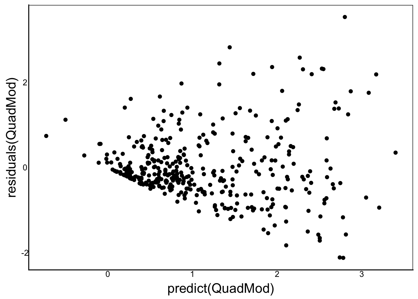

Despite the large number of parameters, our residuals do not give us confidence in the fit of the model. We can try to improve by log-transforming the response variable, or using glm() with family=poisson. This will improve the residuals but the quadratic terms will be complicated to interpret on the scale of \(e^Y\). Another big problem is that our quadratic functions make predictions that are less than zero, but we know we can’t have negative fitness!

GAM

This brings us to generalized additive models. With a simple line of code we can fit a variety of complex functions for each of our phenotypic traits.

We can run simple GAM analyses using the gam() function from the mgcv library.

Since gam is an extension of lm and glm, the formula for coding GAMs is very similar. The main difference is that we want to add a smoothing parameter s() to any predictors where we want to estimate a nonlinear curve:

GAMod<-gam(Fitness ~ s(FlwrAvg) + s(FVegAvg), 
           data=SelDat, method="REML")

The main difference in our model specification is that we have a single, smoothed function s() for each phenotypic trait, rather than linear and quadratic (or higher-order) coefficients. There is a lot of very complicated model fitting going on here. You can get a sense of this if you read through the help ?gam. Luckily, we don’t need to know all the details of the function to run a model and analyze its output. Let’s look at the model summary:

summary(GAMod)

Family: gaussian 
Link function: identity 

Formula:
Fitness ~ s(FlwrAvg) + s(FVegAvg)

Parametric coefficients:
            Estimate Std. Error t value Pr(>|t|)    
(Intercept)  1.12789    0.04562   24.73   <2e-16 ***
---
Signif. codes:  0 '***' 0.001 '**' 0.01 '*' 0.05 '.' 0.1 ' ' 1

Approximate significance of smooth terms:
             edf Ref.df     F p-value    
s(FlwrAvg) 4.917  6.034 20.27  <2e-16 ***
s(FVegAvg) 4.058  5.055 23.02  <2e-16 ***
---
Signif. codes:  0 '***' 0.001 '**' 0.01 '*' 0.05 '.' 0.1 ' ' 1

R-sq.(adj) =   0.37   Deviance explained = 38.5%
-REML = 512.82  Scale est. = 0.797     n = 383

The first thing we see at the top of the output, are the Family and Link functions that make the GAMs Generalized, followed by the formula we defined in our gam function. Next, we see the Parametric coefficients, which are the GAM equivalents of our fixed effects. In this case, just a single overall intercept (mean). In addition, we see the smooting terms s() for each predictor, but rather than separate coefficients like we would get with poly(), we get edf or estimated degrees of freedom. The edf gives us a sense of how ‘wiggly’ the function is, from linear when edf=1 to very convoluted as edf increases. We also have an adjusted R-squared value showing the fit of the model.

IMPORTANT: We should not interpret the p-values in the summary here. As with glm, we should use a likelihood ratio test if we want to know whether a parameter is significant.

Different Intercepts

The above model fits a single curve, but we saw in our linear models that each site has different relationships. Let’s first incorporate different mean fitness at each site.

GAMod2<-gam(Fitness ~ s(FlwrAvg) + s(FVegAvg) + Site, 
            data=SelDat, method="REML")
summary(GAMod2)

Family: gaussian 
Link function: identity 

Formula:
Fitness ~ s(FlwrAvg) + s(FVegAvg) + Site

Parametric coefficients:
              Estimate Std. Error t value Pr(>|t|)    
(Intercept)     0.7897     0.1338   5.903 8.04e-09 ***
Site2_KSR       0.7857     0.1741   4.512 8.63e-06 ***
Site3_Timmins   0.1679     0.2519   0.667    0.505    
---
Signif. codes:  0 '***' 0.001 '**' 0.01 '*' 0.05 '.' 0.1 ' ' 1

Approximate significance of smooth terms:
             edf Ref.df      F  p-value    
s(FlwrAvg) 4.057  5.079  7.737 8.34e-07 ***
s(FVegAvg) 4.657  5.754 22.060  < 2e-16 ***
---
Signif. codes:  0 '***' 0.001 '**' 0.01 '*' 0.05 '.' 0.1 ' ' 1

R-sq.(adj) =  0.422   Deviance explained = 43.8%
-REML = 496.96  Scale est. = 0.73156   n = 383

Note how we now have three Parametric coefficients corresponding to the mean and deviation of each site (e.g. \(43.8\) for the BEF site and \(43.8+45.7=89.5\) for the KSR site).

Now what if we want separate smoothing functions for each site? The obvious solution might be:

Different curves

GAMod3<-gam(Fitness ~ s(FlwrAvg)*Site + s(FVegAvg)*Site, 
            data=SelDat, method="REML")

Warning in sp[i] <- ind: number of items to replace is not a multiple of
replacement length
Warning in sp[i] <- ind: number of items to replace is not a multiple of
replacement length

Error in `model.frame.default()`:
! invalid type (list) for variable 's(FlwrAvg)'

But this generates an error. If we use the help to look at the smoothing function ?s, we can see the solution

GAMod3<-gam(Fitness ~ s(FlwrAvg, by=Site) + 
              s(FVegAvg, by=Site), 
            data=SelDat, method="REML")
summary(GAMod3)

Error in `smoothCon()`:
! Can't find by variable

Error:
! object 'GAMod3' not found

Still another error… looking at the by parameter in ?s we see a clue: by a numeric or factor variable of the same dimension of each covariate. Let’s troubleshoot:

We know the dimension is the same because they are all vectors in the same data frame, with the same number of observations, so the error must be in the type of variable:

is.factor(SelDat$Site)

[1] FALSE

Note that we didn’t have to do this earlier, when we included FlwrAvg:FVegAvg:Site in our quadratic model QuadMod. We can also run a gam with Site as a predictor, without producing an error:

gam(Fitness ~ Site, data=SelDat)

Family: gaussian 
Link function: identity 

Formula:
Fitness ~ Site
Total model degrees of freedom 3 

GCV score: 1.066412     

So it appears to be specifically a problem for the smoothing function s(). We can solve this by using the as.factor() function in s(by=as.factor(Site)) but we know Site should be a factor anyway, so we can just replace the type it in the original dataset:

SelDat$Site<-as.factor(SelDat$Site)
GAMod3<-gam(Fitness ~ s(FlwrAvg, by=Site) + s(FVegAvg, by=Site), 
            data=SelDat, method="REML")
summary(GAMod3)

Family: gaussian 
Link function: identity 

Formula:
Fitness ~ s(FlwrAvg, by = Site) + s(FVegAvg, by = Site)

Parametric coefficients:
            Estimate Std. Error t value Pr(>|t|)    
(Intercept)   1.0357     0.1375   7.532 3.99e-13 ***
---
Signif. codes:  0 '***' 0.001 '**' 0.01 '*' 0.05 '.' 0.1 ' ' 1

Approximate significance of smooth terms:
                           edf Ref.df      F  p-value    
s(FlwrAvg):Site1_BEF     3.104  3.735  3.492 0.020647 *  
s(FlwrAvg):Site2_KSR     4.662  5.513 17.728  < 2e-16 ***
s(FlwrAvg):Site3_Timmins 1.000  1.000 14.852 0.000138 ***
s(FVegAvg):Site1_BEF     1.426  1.736 39.114  < 2e-16 ***
s(FVegAvg):Site2_KSR     5.717  6.692 17.831  < 2e-16 ***
s(FVegAvg):Site3_Timmins 1.872  2.378  0.925 0.484047    
---
Signif. codes:  0 '***' 0.001 '**' 0.01 '*' 0.05 '.' 0.1 ' ' 1

R-sq.(adj) =  0.529   Deviance explained = 55.1%
-REML = 466.94  Scale est. = 0.59578   n = 383

Now look carefully at the smooth terms and compare to the quadratic model (QuadMod) above. Unlike the lm and glm we don’t have an overall intercept and slope with deviations in site means and slope for. Instead, we have a single smoothing term estimated separately for each site. Each smoothing term has a different edf indicating different levels of complexity, with a simple linear relationship (edf=1) for FlwrAvg at the Timmins site.

We can use model selection to compare the GAM with the quadratic model:

AIC(QuadMod) - AIC(GAMod3)

[1] 36.46674

Remember the smaller AIC means a better fit, with a \(\Delta AIC < 2\) being considered equivalent models. In this case the difference is quite large, indicating that GAMod3 is a much better fit to the data. Because gam is ‘generalized’ like glm, we can also try fitting the log-linear (Poisson) model, using a link function for the response variable.

IMPORTANT NOTE: Selection analysis should not be run on transformed data, otherwise the relationship is hard to interpret. When we run a phenotypic selection, we want coefficients that relate standard deviations of a trait value to multiples of mean fitness. However, there are other datasets where a transformation may be appropriate. Let’s quickly look at how we could incorporate other error distributions with the gam function.

Link family

BUT remember that the poisson distribution is for integers, so we need to round our biomass to whole numbers or else we will get a very annoying set of warning messages (one for each row of data). This will lose a small amount of information (tenths of a gram), so just to be safe we’ll make a new column:

SelDat$iFit<-as.integer(SelDat$Fitness)

GAMod4<-gam(iFit ~ s(FlwrAvg, by=Site) + s(FVegAvg, by=Site), 
            family=poisson, data=SelDat, method="REML")
AIC(GAMod3) - AIC(GAMod4)

[1] 226.0945

In this case, we get a large \(\Delta AIC\), indicating a better fit for GAMod4.

Looking back at our Fitness data, we can see that it is mostly the zeros in the northern site.

Zero-inflated

A distribution with an excess of zeros is called zero-inflated and it is both a common and difficult problem with many biological data sets. In our case, we have a number of plants that either died or survived but did not produce viable fruits. These plants are all coded as having zero fitness, giving us something like a bimodal distribution due to the excess zeros:

ggplot(aes(x=Fitness),data=filter(SelDat,Site=="3_Timmins")) + 
         geom_histogram()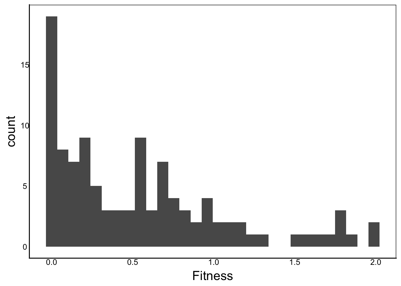

An easy way to deal with zero-inflated data is to split the response variable into two separate data sets – a binary variable and a continuous (Gaussian or Poisson) variable. In our example, we could create a new column called Flowered and recode the fitness to 1 wherever fitness is greater than zero, and zero when fitness is equal to zero. Then, we could analyze Flowered in a logistic regression. We can have a second response variable (e.g. Seeds) that excludes plants with zero fitness, and analyze it with a Gaussian or Poisson error. We just have to be careful how we interpret the results, since the two variables are not independent. Splitting the data like this also adds complication to interpreting how selection acts on phenotypes.

We can get into more advanced models, like zero-inflated gamms with the zipgam https://github.com/AustralianAntarcticDivision/zigam

or the aster package, which allows for more complex analysis of selection: https://doi.org/10.1093/biomet/asm030

These may be useful to you in the future, but you do not need to know them for this course.

For now, we will continue by ignoring the zero-inflated data. In practice, the biggest issue is that our P-values are unreliable, which is less of a problem for model selection.

GAMM

We can also extend GAM to include random effects, which give us Generalized Additive Mixed Models (GAMM). This is an extension of the Generalized Linear Mixed Models (GLMM) that we covered in the Mixed Models Chapter.

The gamm() function from the mgcv library can be used for this.

In our dataset, seed family is a good example of a random effect, since they are sampled randomly from each population. Remember that our maternal family column (Mat) must be coded as a factor, just like we did for Site:

SelDat$Mat<-as.factor(SelDat$Mat)

Before doing this, we should check our sample size:

Nobs<-SelDat %>% group_by(Site,Mat) %>% summarize(N=n()) 
ggplot(aes(x=N),data=Nobs) + geom_histogram() +
  facet_wrap("Site", ncol=1)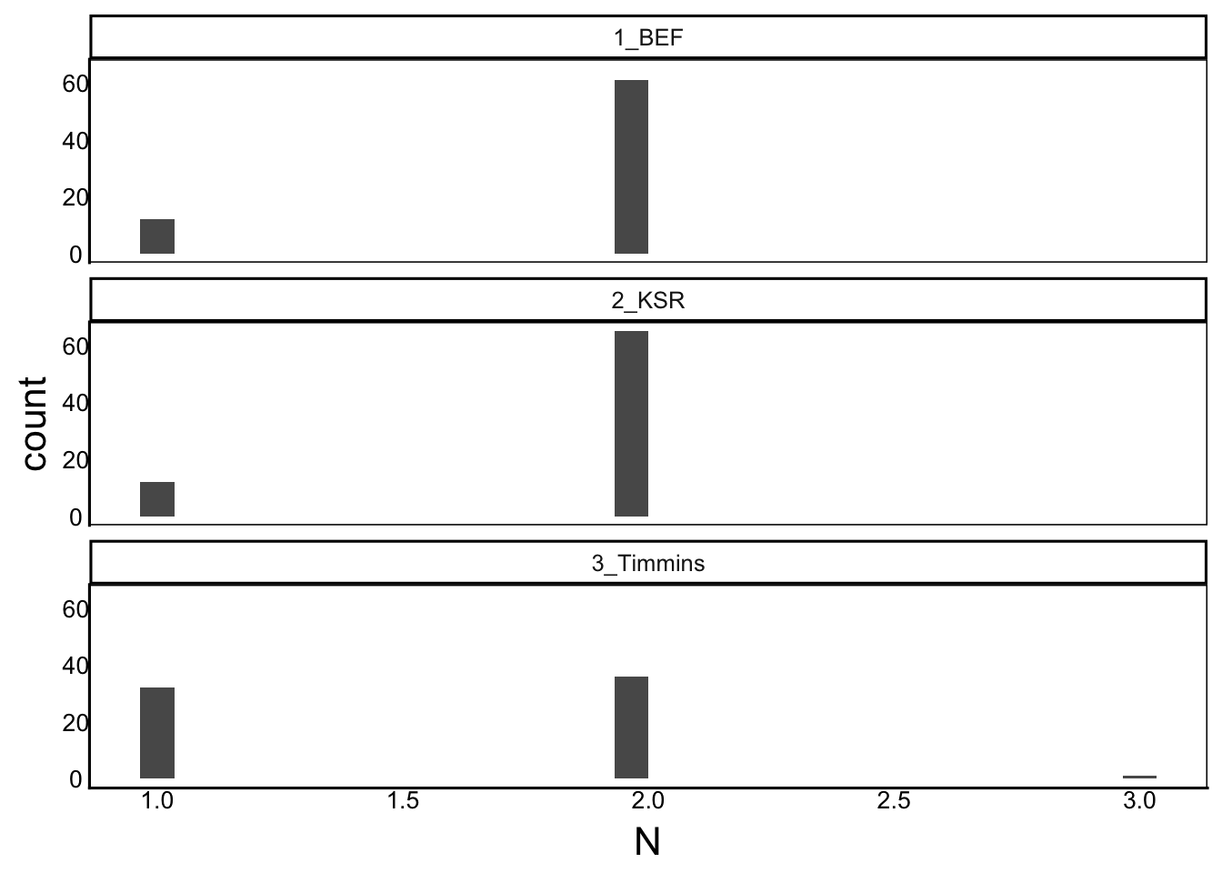

Unfortunately, there is not good replication at the family level (just 1 or 2 surviving plants per family per site). As a result, we will have trouble fitting separate slopes for each family at each site – we would be trying to fit a line to just 1 or 2 points in most cases!

Instead, we can just estimate the variance among family means/intercepts in each garden site:

GAMM<-gamm(Fitness ~ s(FlwrAvg, by=Site) + s(FVegAvg, by=Site), 
            random=list(Mat=~1|Site), data=SelDat, method="REML")

Repeated Measures

In the Mixed Models Chapter, we looked at a type of data called Repeated Measures when the same individuals were measured at different time points. In that tutorial we also looked at a method for fitting random intercepts and slopes. This turns out to be a good fit to the data, but what if the responses over time were nonlinear? In that case we could use a GAMM. The model setup is a bit more complicated though.

First, load the data:

ImmuneDat<-read.csv(
  "https://colauttilab.github.io/Data/ImmuneData.csv",header=T)

Remember in this data set we have paired M-F siblings, with the same IndID, so we should recode.

ImmuneDat$IndID<-paste0(ImmuneDat$IndID,ImmuneDat$Sex)

We’ll also encode the ID variables and Sex as factors to avoid errors:

ImmuneDat<-ImmuneDat %>%
  mutate(FamID=as.factor(FamID),
         IndID=as.factor(IndID),
         Sex=as.factor(Sex))

There’s a few different random models we could use here. First, let’s imagine that we are geneticists so we are interested in these specific genetic families. For example, we might want to see how different families respond over time and then follow-up with genetic screening to identify candidate genes. In this case, we should treat FamID as a fixed effect, with individuals as random effects because they are randomly chosen from each family.

So now we want to estimate separate curves for each family:

GAMi<-gam(IgG ~ FamID + s(Time,by=FamID), data=ImmuneDat)

AND we want to account for random variation among individuals. For this, we use a bs="fs" parameter in the smoothing function. This is a bit different to the other kinds of mixed models.

GAM for Big Data

One drawback of gam is that it is computationally much more intensive than glm, making it inefficient for large datasets. However, the bam() function from the same mgcv package is similar to gamand gamm but optimized for larger datasets.

Note that this can take a long time to run!

BAMi<-bam(IgG ~ FamID + s(Time,by=FamID) + 
              s(Time, IndID, bs="fs"), data=ImmuneDat)