Mixed Models

Introduction

So far, we’ve seen how Linear Models (LM) are a general class of statistical models that include a number of classical models with different names (e.g. ANOVA, Regression), all of which we can run in R with the lm() function. We then generalized from the lm() linear model framework to run Generalized Linear Models (GLM) with glm() that allow us to analyze response variables that are drawn from other distributions including Gaussian, binomial, Poisson – each with pseudo equivalents for over-dispersed error. In practice, it can be difficult to know which error family to use in our model, but we can use model selection to compare models with different family functions, visually inspecting the residual error to make sure the ‘best’ model is behaving well.

In this tutorial, we expand the Generalized Linear Models to include a new kind of estimate called a Random Effect. The “Effects” are the estimates of the predictor variable(s) as shown in the model outputs in R. The Fixed vs Random effects differ in the way these estimates are calculated. To understand the difference, we first define the estimates used in lm and glm as Fixed Effects and then incorporate random effects for comparison.

Fixed or Random?

To determine whether a predictor should be a fixed or random effect, ask yourself two questions:

Is my hypothesis about these specific groups or estimates?

If yes, then this predictor is a fixed effect.

Are these groups or estimates repesentative of a larger population of possible groups?

If yes, then the predictor is a random effect.

Setup

Load libraries and custom plotting theme

library(ggplot2) # plotting library

Warning: package 'ggplot2' was built under R version 4.5.2

library(dplyr) # data management

source("http://bit.ly/theme_pub") # Set custom plotting theme
theme_set(theme_pub())

Mixed Models Packages

There are two popular packages available for mixed models in R. They have different syntax and slighlty different implementation. There is also a package called GLMMadaptive, which is optimized for Generalized Linear Mixed Models (GLMM) aka GL Mixed Effects (GLME) models. We’ll use lme4 for this tutorial, but if you have trouble with it in the ‘real world’, you can try nlme and/or GLMMadaptive.

library(lme4)

Warning: package 'lme4' was built under R version 4.5.2

Loading required package: Matrix

And we’ll do some model selection using likelihood ratio tests, which uses the lrtest() function from the lmtest package

library(lmtest)

Loading required package: zoo

Warning: package 'zoo' was built under R version 4.5.2


Attaching package: 'zoo'

The following objects are masked from 'package:base':

    as.Date, as.Date.numeric

Data

Load the dataset

ImmuneDat<-
  read.csv("https://colauttilab.github.io/Data/ImmuneData.csv",
           header=T)

Inspect the Data:

str(ImmuneDat)

'data.frame':   4860 obs. of  5 variables:
 $ FamID: int  1 1 1 1 1 1 1 1 1 1 ...
 $ IndID: int  16 16 16 16 16 16 16 16 16 16 ...
 $ Time : int  0 1 2 3 4 5 6 7 8 9 ...
 $ Sex  : chr  "M" "M" "M" "M" ...
 $ IgG  : num  141 137 133 129 123 ...

This data measures the immune response to a vaccine given to 135 individuals, measured as the blood-level Immunoglobulin G (IgG) sampled in each patient over 18 months.

IndID – A unique identifier for each patient
FamID – The family ID of each patient. Several individuals come from the same extended family; in this case, individuals with the same FamID share the same maternal grandmother.
Time – Month of measurement from 0 to 17
Sex – Male or Female in this dataset
IgG – Concentration of IgG in the blood

Repeated Measures

Take a careful look at the structure (e.g. str, head) of the data set and you’ll see something that is different from most of the other datasets we’ve looked at.

In the past examples, each row would contain observations for an individual (e.g. individual or pot), and each measurement would have its own column (e.g. size or biomass). This is sometimes called the ‘wide’ format’.

In this dataset, each individual is measured at 18 different time points (\(t = 0\) to \(t = 17\)). If you think of each time point as a separate column, then you might have each individual as a row and each time point as a column. But, we have something different here. Each row contains the measurement of an individual at a specific time point, so each individual has 18 rows. This is sometimes called the ‘long’ format. As covered in the Data Science chapter of the R Crash Course textbook, we can use pivot_wider() and pivot_longer() from the tidyr package to transform our dataset to the wide and long formats, respectively.

This specific data setup is called a Repeated Measures design because measurements are repeated down rows with the same subject ID. In this case, we have multiple time measurements, but we would have a repeated measures design if we measured different traits on the same individuals – for example, if we measured several different metabolites in the blood. These measurements are not independent of each other, because each individual is measured several times.

Repeated measures are a good example of pseudoreplication. As discussed in the Experimental Design Chapter, a pseudoreplicated study or data set has a sample size that is inflated because observations are not independent. In theory, we should take measurements on different individuals if we are going to do a traditional linear model. However, this won’t allow us to identify overall trends across individuals. Luckily, we can used mixed models to account for non-independence of measurements.

Fixed Effects

Both the lm and glm tutorials use fixed effects, we just didn’t call them that. The effects are fixed because we are interested in the specific estimates that are fit to the data.

For example, we might run a linear model to look at sex differences in IgG at time = 0, when the blood concentration is highest. By looking at only the initial timepoint we can avoid problems of repeated measures on the same individual.

InitIgG<-ImmuneDat %>% 
  filter(Time==0)
  
LMod<-lm(IgG ~ Sex,InitIgG)
summary(LMod)


Call:
lm(formula = IgG ~ Sex, data = InitIgG)

Residuals:
     Min       1Q   Median       3Q      Max 
-13.5840  -4.9213  -0.5501   4.7680  13.7295 

Coefficients:
            Estimate Std. Error t value Pr(>|t|)    
(Intercept) 139.9182     0.5291 264.456   <2e-16 ***
SexM          2.0334     0.7482   2.718    0.007 ** 
---
Signif. codes:  0 '***' 0.001 '**' 0.01 '*' 0.05 '.' 0.1 ' ' 1

Residual standard error: 6.147 on 268 degrees of freedom
Multiple R-squared:  0.02682,   Adjusted R-squared:  0.02319 
F-statistic: 7.386 on 1 and 268 DF,  p-value: 0.007003

anova(LMod)

Analysis of Variance Table

Response: IgG
           Df  Sum Sq Mean Sq F value   Pr(>F)   
Sex         1   279.1  279.11  7.3857 0.007003 **
Residuals 268 10127.7   37.79                    
---
Signif. codes:  0 '***' 0.001 '**' 0.01 '*' 0.05 '.' 0.1 ' ' 1

We have a significant effect of Sex on immune response… But another key assumption of independent data points is violated in this model. We are treating each individual as an independent data point but we have genetic relatives. Two individuals from the same genetic family are genetically more similar than two individuals drawn at random. AND we would expect people from the same family to have a more similar response than two individuals chosen at random.

This is another good example of pseudoreplication, but instead of multiple measurements on the same individual, we have multiple measurements of different individuals from the same genetic family.

We can summarize the data to see this:

InitIgG %>% 
  group_by(FamID) %>%
  summarize(n=length(IgG))

# A tibble: 8 × 2
  FamID     n
  <int> <int>
1     1    34
2     2    30
3     3    34
4     4    37
5     5    33
6     6    41
7     7    35
8     8    26

In the classic linear model framework, we could include family as a factor in our model:

LMod2<-lm(IgG ~ Sex + FamID, data=InitIgG)
summary(LMod2)


Call:
lm(formula = IgG ~ Sex + FamID, data = InitIgG)

Residuals:
     Min       1Q   Median       3Q      Max 
-13.8181  -4.9210  -0.5844   4.7924  13.3247 

Coefficients:
            Estimate Std. Error t value Pr(>|t|)    
(Intercept) 140.7001     0.9369 150.175  < 2e-16 ***
SexM          1.9980     0.7490   2.668  0.00811 ** 
FamID        -0.1708     0.1689  -1.011  0.31283    
---
Signif. codes:  0 '***' 0.001 '**' 0.01 '*' 0.05 '.' 0.1 ' ' 1

Residual standard error: 6.147 on 267 degrees of freedom
Multiple R-squared:  0.03053,   Adjusted R-squared:  0.02327 
F-statistic: 4.204 on 2 and 267 DF,  p-value: 0.01593

anova(LMod2)

Analysis of Variance Table

Response: IgG
           Df  Sum Sq Mean Sq F value   Pr(>F)   
Sex         1   279.1 279.106  7.3864 0.007002 **
FamID       1    38.6  38.640  1.0226 0.312826   
Residuals 267 10089.0  37.787                    
---
Signif. codes:  0 '***' 0.001 '**' 0.01 '*' 0.05 '.' 0.1 ' ' 1

CODING ERROR!

Hold on a sec, there’s something VERY wrong here in our summary output!

Question: What is the problem with the output, above? Find the error before proceeding

Hint: check the degrees of freedom

Answer: We have 8 families, which means we should have 7 estimates in our summary (intercept + 7 means). But we only have one estimate for FamID – why??

This is a very common mistake and it occurs because of an error in the way we have defined our variables. Let’s look again at the structure of our data:

str(InitIgG)

'data.frame':   270 obs. of  5 variables:
 $ FamID: int  1 1 1 1 1 1 1 1 1 1 ...
 $ IndID: int  16 19 22 22 26 26 27 30 32 34 ...
 $ Time : int  0 0 0 0 0 0 0 0 0 0 ...
 $ Sex  : chr  "M" "F" "M" "F" ...
 $ IgG  : num  141 133 132 140 140 ...

FamID and IndID are integers because when R analyzed our data it treated this integer column as a continuous variable, rather than a categorical variable. In contrast, Sex is a string because it has two letter: M or F. By default, R treats integers as continuous data and strings as factors. So we need to redefine our ID columns as factors.

InitIgG<-InitIgG %>% 
  mutate(IndID=as.factor(IndID),
         FamID=as.factor(FamID),
         Sex=as.factor(Sex))
str(InitIgG)

'data.frame':   270 obs. of  5 variables:
 $ FamID: Factor w/ 8 levels "1","2","3","4",..: 1 1 1 1 1 1 1 1 1 1 ...
 $ IndID: Factor w/ 135 levels "1","2","3","4",..: 16 19 22 22 26 26 27 30 32 34 ...
 $ Time : int  0 0 0 0 0 0 0 0 0 0 ...
 $ Sex  : Factor w/ 2 levels "F","M": 2 1 2 1 2 1 2 1 2 2 ...
 $ IgG  : num  141 133 132 140 140 ...

Now we can see there are 8 families and 135 individuals

Don’t forget to fix the original data set too!

ImmuneDat<-ImmuneDat %>% 
  mutate(IndID=as.factor(IndID),
         FamID=as.factor(FamID),
         Sex=as.factor(Sex))

Correct LM

Now our model should work properly

LMod2<-lm(IgG ~ Sex + FamID, data=InitIgG)
summary(LMod2)


Call:
lm(formula = IgG ~ Sex + FamID, data = InitIgG)

Residuals:
    Min      1Q  Median      3Q     Max 
-10.792  -2.215  -0.049   2.191  12.207 

Coefficients:
            Estimate Std. Error t value Pr(>|t|)    
(Intercept) 137.7451     0.6501 211.887  < 2e-16 ***
SexM          2.8433     0.4323   6.577 2.60e-10 ***
FamID2        9.7281     0.8842  11.002  < 2e-16 ***
FamID3       -5.0561     0.8535  -5.924 9.90e-09 ***
FamID4       -2.0199     0.8362  -2.416 0.016398 *  
FamID5        8.4572     0.8606   9.828  < 2e-16 ***
FamID6        5.5543     0.8169   6.800 7.12e-11 ***
FamID7        0.3694     0.8502   0.434 0.664288    
FamID8       -3.3663     0.9172  -3.670 0.000294 ***
---
Signif. codes:  0 '***' 0.001 '**' 0.01 '*' 0.05 '.' 0.1 ' ' 1

Residual standard error: 3.519 on 261 degrees of freedom
Multiple R-squared:  0.6894,    Adjusted R-squared:  0.6799 
F-statistic: 72.41 on 8 and 261 DF,  p-value: < 2.2e-16

anova(LMod2)

Analysis of Variance Table

Response: IgG
           Df Sum Sq Mean Sq F value    Pr(>F)    
Sex         1  279.1  279.11  22.537 3.402e-06 ***
FamID       7 6895.3  985.04  79.537 < 2.2e-16 ***
Residuals 261 3232.4   12.38                      
---
Signif. codes:  0 '***' 0.001 '**' 0.01 '*' 0.05 '.' 0.1 ' ' 1

In this case, the estimate of the Sex effect is different and the p-value for the Sex effect is much smaller (i.e. more significant). We also have a much larger Adjusted R-squared, meaning that the model explains more of the variation in the data (ie., less residual error). This gives us more statistical power to detect biological effects. We can also see that some families are significantly different from the intercept but others are not.

This is a better model but we have two more problems. First, we have to estimate several parameters, which takes more degrees of freedom, and therefore reduces the statistical power of our model. It gets even worse if we want to test whether the difference between sexes is different for each family:

LMod3<-lm(IgG ~ Sex*FamID, data=InitIgG)
summary(LMod3)


Call:
lm(formula = IgG ~ Sex * FamID, data = InitIgG)

Residuals:
     Min       1Q   Median       3Q      Max 
-11.2438  -2.1036   0.1046   2.2422  12.7921 

Coefficients:
            Estimate Std. Error t value Pr(>|t|)    
(Intercept) 138.6188     0.8952 154.844  < 2e-16 ***
SexM          1.2797     1.1975   1.069 0.286278    
FamID2        7.7826     1.2121   6.421 6.63e-10 ***
FamID3       -6.3871     1.2660  -5.045 8.64e-07 ***
FamID4       -2.0357     1.2660  -1.608 0.109098    
FamID5        6.6661     1.2282   5.427 1.33e-07 ***
FamID6        4.2499     1.1721   3.626 0.000348 ***
FamID7        0.3403     1.1721   0.290 0.771830    
FamID8       -3.6962     1.3138  -2.813 0.005287 ** 
SexM:FamID2   4.2428     1.7617   2.408 0.016739 *  
SexM:FamID3   2.3819     1.6936   1.406 0.160813    
SexM:FamID4   0.1206     1.6679   0.072 0.942403    
SexM:FamID5   3.4556     1.7008   2.032 0.043218 *  
SexM:FamID6   2.4463     1.6148   1.515 0.131034    
SexM:FamID7  -0.5480     1.6927  -0.324 0.746404    
SexM:FamID8   0.4757     1.8121   0.263 0.793120    
---
Signif. codes:  0 '***' 0.001 '**' 0.01 '*' 0.05 '.' 0.1 ' ' 1

Residual standard error: 3.467 on 254 degrees of freedom
Multiple R-squared:  0.7066,    Adjusted R-squared:  0.6893 
F-statistic: 40.78 on 15 and 254 DF,  p-value: < 2.2e-16

anova(LMod3)

Analysis of Variance Table

Response: IgG
           Df Sum Sq Mean Sq F value    Pr(>F)    
Sex         1  279.1  279.11 23.2178 2.491e-06 ***
FamID       7 6895.3  985.04 81.9418 < 2.2e-16 ***
Sex:FamID   7  179.0   25.57  2.1271   0.04132 *  
Residuals 254 3053.4   12.02                      
---
Signif. codes:  0 '***' 0.001 '**' 0.01 '*' 0.05 '.' 0.1 ' ' 1

Now we have 14 parameters – and we’re still only looking at one time point. If we wanted to fit a linear regression over time, we would need 8 more parameters for slope (one overall slope + 7 slope deviations). If we wanted to fit a quadratic (curved) response over time then we would need another 8 estimates for the squared (quadratic) term. That would be:

1 intercept +
1 regression slope +
1 quadratic slope +
7 group means +
7 group:sex means (intercepts) +
7 linear slopes +
7 quadratic slopes

That’s 30 parameters!

Too many parameters is one problem. Another problem is the fact that we don’t have a balanced sample (compare N of individuals for each family, above). When our samples are imbalanced, we can get big standard errors on our estimates, making them unreliable for families with smaller sample sizes.

A third problem would arise if families differ in their variability. For example, imagine there is a gene that regulates the immune response, so that if we look at the variability in response among individuals, some families have a more variable response, and some have a less variable response. This would be heteroskedasticity – another violation of linear models.

Finally, there is a conceptual problem: We aren’t really interested in these specific families. Instead, we might assume that we randomly sampled these from a much large population of all potential human families. The above models don’t account for the random sampling of genetic families, only the residual error among randomly sampled individuals.

Random effects solve all three of these problems.

Random Effects

A random effect assume that the levels of a predictor are chosen at random from a larger population. Just as we sampled individual observations from a larger population in the Distributions Chapter we can sample genetic families from a larger population of genetic families, and we can sample individuals within a family from a larger population of individuals from the same family.

That’s where the term ‘random effects’ comes from: we are assuming that the different levels of a random effect are a random, unbiased sample from a larger population of effects.

Instead of estimating each individual mean for a random effect, we assume the effects are drawn from a random distribution. As a result, we estimate a single term – the variance – rather than a separate term for the effect of each family.

Linear Mixed Model

The Linear Mixed Model (LMM), aka the Linear Mixed Effects (LME) model is just a Linear Model (LM) with the addition of random effects.

To run LMEs we will use the lmer() function from the lme4 package. Another popular package is nlme The syntax is the same for the fixed effects but the random effects get a bit more complicated.

For now, let’s ignore sex-by-family interactions and do the mixed-model equivalent of the linear model for sex + family effects:

MMod<-lmer(IgG ~ Sex + (1 | FamID), data=InitIgG)
summary(MMod)

Linear mixed model fit by REML ['lmerMod']
Formula: IgG ~ Sex + (1 | FamID)
   Data: InitIgG

REML criterion at convergence: 1475.7

Scaled residuals: 
    Min      1Q  Median      3Q     Max 
-3.0542 -0.6357 -0.0115  0.6124  3.4583 

Random effects:
 Groups   Name        Variance Std.Dev.
 FamID    (Intercept) 30.27    5.502   
 Residual             12.38    3.519   
Number of obs: 270, groups:  FamID, 8

Fixed effects:
            Estimate Std. Error t value
(Intercept) 139.4593     1.9691  70.824
SexM          2.8331     0.4323   6.554

Correlation of Fixed Effects:
     (Intr)
SexM -0.109

Compare the above with the lm() summary earlier. It’s important to take time to inspect and understand the similarities and differences:

First, look at the Fixed Effects. Compare the Estimate for the Intercept and SexM to the analogous estimates in the linear model lm(IgG ~ Sex + FamID), which we ran earlier.

Second, look at the Random Effects in this model. Notice how there are no individual estimates for FamID, just a single (Intercept) term, which is actually a Variance rather than a mean or slope as we would get in a fixed effect estimate. Note that there is also a Residual variance term in our random effects, which is an estimate of the residual error variance among individuals.

Variance Components

You can think of random effects like an ANOVA in the sense that we are trying to account for variance of each predictor. However, unlike ANOVA we are estimating the variance directly from the data, rather estimating means for each group and then calculating the sums of squares among group means.

Those predictors can be independent of each other, or they can be hierarchical. Hierarchical random effects are called Nested effects. An example of a nested effect would be if several genetic families were randomly sampled from each of several randomly selected populations. Or in our cases, individuals were randomly sampled from each genetic family.

Computationally, nested effects just avoid a simple problem with coding. In our example, each individual ID is unique, but sometimes they might be coded using non-unique identifiers. For example, compare these two tables showing two different ways of coding family and ID codes:

Non-unique ID

Family	Individual
1	1
1	2
1	3
2	1
2	2
2	3
2	4

Unique ID

Family	Individual
1	1
1	2
1	3
2	4
2	5
2	6
2	7

CODING CAUTION!

In both cases, we have 7 different individuals, representing 2 families. Now think about what would happen if we included Individual as a random effect (ignoring family for now).

In the second example, we would estimate the variance among 7 individuals, but in the first example, we would estimate the variance among 4 individuals. THIS WOULD BE WRONG! It would happen because R would see the same ID code for individual 1 from each family as being the same individual, but in fact they are different individuals

In R, the easiest way to avoid this mistake, is to just recode each individual with a unique ID.

Multiple Factors

Returning to the dataset, we can consider other mixed models. Let’s consider the interaction model:

formula(LMod3)

IgG ~ Sex * FamID

Question: What is the mixed model equivalent?

With mixed models we are estimating the variance components. We already estimated the variance among families as (1|FamID) and we had sex as a fixed effect. So we just need the MME equivalent of the interaction term. If there is a significant interaction term in a linear model, it would mean that the difference between males and females differs for each family. Since families are randomly sampled, another way to think of this is that the variance among families differs for males and females, which we can add to the model:

MMod2<-lmer(IgG ~ Sex + (Sex | FamID) , data=InitIgG)
summary(MMod2)

Linear mixed model fit by REML ['lmerMod']
Formula: IgG ~ Sex + (Sex | FamID)
   Data: InitIgG

REML criterion at convergence: 1468.7

Scaled residuals: 
    Min      1Q  Median      3Q     Max 
-3.2261 -0.5837 -0.0305  0.6386  3.6242 

Random effects:
 Groups   Name        Variance Std.Dev. Corr 
 FamID    (Intercept) 24.052   4.904         
          SexM         1.706   1.306    0.95 
 Residual             12.024   3.468         
Number of obs: 270, groups:  FamID, 8

Fixed effects:
            Estimate Std. Error t value
(Intercept) 139.5133     1.7597  79.282
SexM          2.8187     0.6285   4.485

Correlation of Fixed Effects:
     (Intr)
SexM 0.605

Compare the Random effects in this model to the one with only a single random effect (1|FamID). In this model we have a second variance component, which is the additional variance explained by separating Males and Females.

It’s also important to note that we also have Sex in the Fixed effects, which is still the deviation from the intercept in the average IgG of Males. So we include Sex as both a fixed effect and a random effect in the model. In the fixed term, we estimate the deviation in the mean for the group, but in the random effect we use it to subdivide the among-family variance separately for male and female offspring.

Note that this variance is very small, meaning that separating families by sex doesn’t explain a lot more of the variation. Also notice that the residual variance is almost the same – most of the variance explained by SexM comes out of the family variance.

So is sex a significant predictor? We can test its significance using model selection:

lrtest(MMod2,MMod)

Likelihood ratio test

Model 1: IgG ~ Sex + (Sex | FamID)
Model 2: IgG ~ Sex + (1 | FamID)
  #Df  LogLik Df  Chisq Pr(>Chisq)  
1   6 -734.35                       
2   4 -737.83 -2 6.9673    0.03069 *
---
Signif. codes:  0 '***' 0.001 '**' 0.01 '*' 0.05 '.' 0.1 ' ' 1

We can also test the significance of Sex as a fixed effect by comparing to a model with a single intercept rather than separate estimates for each sex:

MMod3<-lmer(IgG ~ 1 + (Sex | FamID), data=InitIgG)
lrtest(MMod2,MMod3)

Likelihood ratio test

Model 1: IgG ~ Sex + (Sex | FamID)
Model 2: IgG ~ 1 + (Sex | FamID)
  #Df  LogLik Df  Chisq Pr(>Chisq)    
1   6 -734.35                         
2   5 -740.16 -1 11.619  0.0006529 ***
---
Signif. codes:  0 '***' 0.001 '**' 0.01 '*' 0.05 '.' 0.1 ' ' 1

We can see a highly significant effect.

Random Regression

So far we have looked at just one time point in our data, with family as a random effect, but we are ignoring most of our data! Our Time column shows the number of months since vaccination, so we can treat it as a continuous variable and try to fit a statistical model. To do this, we need some kind of regression function for the change in IgG over time. If we just plot the raw data:

ggplot(aes(x=Time, y=IgG), data=ImmuneDat) +
  geom_point() + 
  geom_smooth()

`geom_smooth()` using method = 'gam' and formula = 'y ~ s(x, bs = "cs")'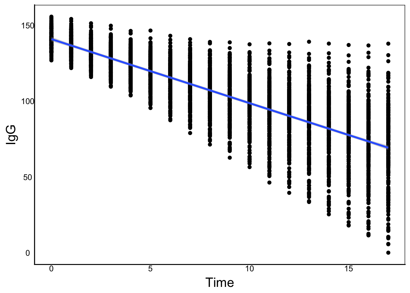

We can see that there is a general linear decline, but also an increase in variance. We can plot individual curves to get a sense of the overall relationship that we can try to model:

ggplot(aes(x=Time, y=IgG, group=IndID), data=ImmuneDat) +
  geom_point() + 
  geom_smooth()

`geom_smooth()` using method = 'loess' and formula = 'y ~ x'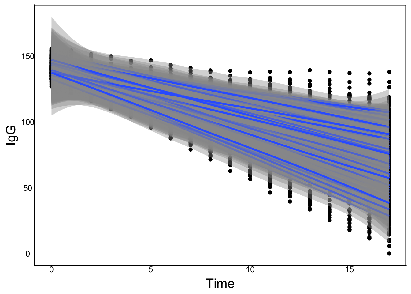

We can see how different individuals have different slopes and intercepts. Different families could also have different linear relationships like this. We can try to fit a simple linear regression model and look at the residuals:

LReg<-lm(IgG ~ FamID*Time + IndID*Time, 
         data=ImmuneDat)
ggplot()+
  geom_point(aes(predict(LReg),residuals(LReg)))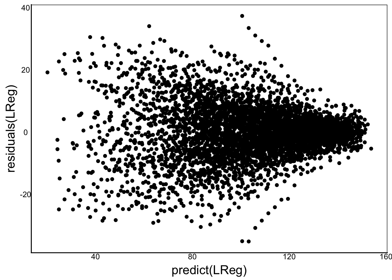

It doesn’t look too bad, but overall the residuals are centered around zero but seem to be heteroskedastic (unequal variance) along our predictors. Let’s try building a mixed model and then come back to compare the residuals. From the graphs above, we can see that a simple linear regression is a good function to use for time. Let’s start with the simplest model by incorporating time as a fixed effect:

MModTime<-lmer(IgG ~ Sex * Time + (1  | FamID), 
               data=ImmuneDat)
summary(MModTime)

Linear mixed model fit by REML ['lmerMod']
Formula: IgG ~ Sex * Time + (1 | FamID)
   Data: ImmuneDat

REML criterion at convergence: 37781.7

Scaled residuals: 
    Min      1Q  Median      3Q     Max 
-4.2347 -0.5411  0.0152  0.5715  4.3030 

Random effects:
 Groups   Name        Variance Std.Dev.
 FamID    (Intercept) 127.4    11.29   
 Residual             137.8    11.74   
Number of obs: 4860, groups:  FamID, 8

Fixed effects:
             Estimate Std. Error t value
(Intercept) 138.99610    4.01757  34.597
SexM          2.93493    0.64799   4.529
Time         -3.72939    0.04590 -81.257
SexM:Time    -0.97904    0.06491 -15.084

Correlation of Fixed Effects:
          (Intr) SexM   Time  
SexM      -0.081              
Time      -0.097  0.602       
SexM:Time  0.069 -0.851 -0.707

Note that we get a single slope for our fixed effect of Time, and another for the change in slope for male vs. female patients. These represent the overall average effect of how IgG changes over time. Since the estimate for time is negative, it shows that, on average, IgG levels decline over time. Since the SexM:Time is also negative, the decline is slightly faster for males – though we should test whether this is significant using the LRT. We won’t do it here, because you should know how to do this by now. Review the Model Selection Chapter and the above examples above as a guide.

The next thing we can do is account for different relationships for each genetic family:

MModTime2<-lmer(IgG ~ Sex * Time + (Time| FamID), data=ImmuneDat)
summary(MModTime2)

Linear mixed model fit by REML ['lmerMod']
Formula: IgG ~ Sex * Time + (Time | FamID)
   Data: ImmuneDat

REML criterion at convergence: 37163.3

Scaled residuals: 
    Min      1Q  Median      3Q     Max 
-4.7957 -0.4904  0.0319  0.5198  4.2896 

Random effects:
 Groups   Name        Variance Std.Dev. Corr 
 FamID    (Intercept)  29.426   5.4246       
          Time          0.797   0.8927  0.49 
 Residual             120.760  10.9891       
Number of obs: 4860, groups:  FamID, 8

Fixed effects:
            Estimate Std. Error t value
(Intercept) 139.4491     1.9656  70.944
SexM          2.6906     0.6104   4.408
Time         -3.7826     0.3186 -11.873
SexM:Time    -0.9508     0.0613 -15.511

Correlation of Fixed Effects:
          (Intr) SexM   Time  
SexM      -0.155              
Time       0.450  0.082       
SexM:Time  0.132 -0.853 -0.096

Note that the fixed effect of Time is the overall slope, but the random effecst of Time include:

(Intercept) – the variance in intercept among families
Time – the variance in slope among families.

lrtest(MModTime,MModTime2)

Likelihood ratio test

Model 1: IgG ~ Sex * Time + (1 | FamID)
Model 2: IgG ~ Sex * Time + (Time | FamID)
  #Df LogLik Df  Chisq Pr(>Chisq)    
1   6 -18891                         
2   8 -18582  2 618.43  < 2.2e-16 ***
---
Signif. codes:  0 '***' 0.001 '**' 0.01 '*' 0.05 '.' 0.1 ' ' 1

Now we see highly significant improvement in the fit of the model, and new Random effects for Intercept and Time. Again, note that there is just one estimate for each, representing the variance among intercepts and slopes across all of the families. Also note that the difference in degrees of freedom is 2, even though the first model also had a random effect for family ID. In addition to the random slope, we also estimate a correlation among families between the slope and intercept. We do this because the two estimates are not independent – think about how the intercept changes as you vary the slope for a given set of data.

ML vs ReML

Mixed effects models are fit using a method called Maximum Likelihood (ML) or often Restricted Maximum Likelihood (ReML) when we include random effects. This is usually done computationally and it’s related to the ‘likelihood’ scores that we discussed in the Model Selection Chapter. Remember that a model’s likelihood (\(\theta\)) is the probability of observing the data given a particular statistical model.

The difference here is that we have a computational algorithm that searches a range of estimates (e.g. variance components), and then chooses the values that maximize the likelihood of the model given the data. It’s sort of like doing a whole bunch of model selection iterations with slightly different estimates and then considering the best fit. In other words, the algorithm finds the parameter values that are the best fit to the data. ReML is similar to ML except that the model estimates are ‘restricted’ to not have negative variances. It has been shown that ReML estimates are less biased than ML when sample sizes are unequal or small.

Maximum likelihood (and ReML) is a powerful method for model fitting, but it does have some limitations, which we explore below.

Convergence Error

Looking back at our data, we can also try to calculate a separate slope for each individual, not just each family. Again, here we would calculate the variance of the intercept and slopes across all individuals, rather than estimating specific intercepts and slopes:

MModTime3<-lmer(IgG ~ Sex * Time + (1 +  Time| FamID) + 
                  (1 + Time |IndID), data=ImmuneDat)

Warning in checkConv(attr(opt, "derivs"), opt$par, ctrl = control$checkConv, : Model failed to converge with max|grad| = 0.00208158 (tol = 0.002, component 1)
  See ?lme4::convergence and ?lme4::troubleshooting.

Here we get an important error: “Model failed to converge”.

This means that our model is unreliable because there are several different parameter values that give similar likelihood scores. This usually happens for two reasons:

Model specification error: This happens when we try to estimate too many parameters and we don’t have enough residual degrees of freedom. For example, if each genetic family was also from a different population, we wouldn’t be able to include both family and population as separate random effects because we wouldn’t be able to estimate separate variance components. This is similar to the collinearity problem with linear models, except that it happens with the grouping variable of the random effects. We avoid this problem by thinking carefully about our experimental design and limitations imposed bby the data.
Too much parameter space: Sometimes there is just a lot of different parameter values that need to be tested to find the maximum likelihood. In other wods, there are different combinations of estimates that fit the data equally well. We can try to help the searching algorithm by setting the start= parameters, and/or we reduce the number of predictors in our model.

In both cases, We can get some insight into the model performance with the verbose=T parameter.

MModTime3<-lmer(IgG ~ Sex * Time + (1 +  Time| FamID) + 
                  (1 + Time |IndID), data=ImmuneDat, verbose=T)

The output (not shown) shows the fit (log likelihood) of the model for each iteration of the search algorithm. From this we can see that it declines quickly for the first ~100 iterations before getting ‘stuck’ without much improvement in fit.

It appears we have a problem estimating separate slopes for each individual. The reason goes back to the way we define our random effect of IndID and the way it is encoded in the data. For example, let’s look at th data for IndID==1

Ind1<-ImmuneDat %>%
  filter(IndID=="1")
ggplot(aes(x=Time,y=IgG,colour=Sex), data=Ind1) +
  geom_point()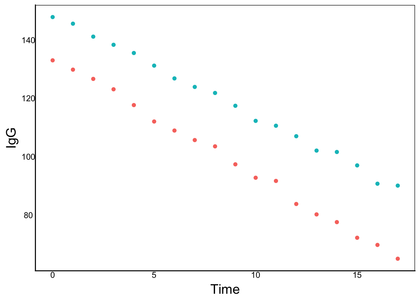

We can see that there is a big coding error in our dataset! Each IndID is not a unique individual – it is actually two individuals – one male and one female. In this case, they are siblings (brother and sister). When we use IndID as a random effect in the mixed model, we are trying to fit a single slope for two different individuals. What we want to do is recode the IndID so that each INDIVIDUAL has a unique ID. But another way we can deal with this is to nest individual within sex. In R we use the backslash (/) to define nested terms:

MModTime4<-lmer(IgG ~ Sex * Time + (1 + Time|FamID) +
                  (1 + Time|IndID/Sex), data=ImmuneDat)

boundary (singular) fit: see help('isSingular')

summary(MModTime4)

Linear mixed model fit by REML ['lmerMod']
Formula: IgG ~ Sex * Time + (1 + Time | FamID) + (1 + Time | IndID/Sex)
   Data: ImmuneDat

REML criterion at convergence: 17845.3

Scaled residuals: 
    Min      1Q  Median      3Q     Max 
-3.7369 -0.6437 -0.0151  0.6267  3.4704 

Random effects:
 Groups    Name        Variance Std.Dev. Corr  
 Sex:IndID (Intercept) 11.56828 3.4012         
           Time         1.10025 1.0489   -0.01 
 IndID     (Intercept)  0.00000 0.0000         
           Time         0.03182 0.1784    NaN  
 FamID     (Intercept) 29.78677 5.4577         
           Time         0.76202 0.8729   0.48  
 Residual               1.21692 1.1031         
Number of obs: 4860, groups:  Sex:IndID, 270; IndID, 135; FamID, 8

Fixed effects:
            Estimate Std. Error t value
(Intercept) 139.4470     1.9524  71.422
SexM          2.7065     0.4222   6.410
Time         -3.7807     0.3221 -11.737
SexM:Time    -0.9510     0.1290  -7.374

Correlation of Fixed Effects:
          (Intr) SexM   Time  
SexM      -0.108              
Time       0.456  0.003       
SexM:Time  0.002 -0.016 -0.199
optimizer (nloptwrap) convergence code: 0 (OK)
boundary (singular) fit: see help('isSingular')

lrtest(MModTime2,MModTime4)

Likelihood ratio test

Model 1: IgG ~ Sex * Time + (Time | FamID)
Model 2: IgG ~ Sex * Time + (1 + Time | FamID) + (1 + Time | IndID/Sex)
  #Df   LogLik Df Chisq Pr(>Chisq)    
1   8 -18581.6                        
2  14  -8922.6  6 19318  < 2.2e-16 ***
---
Signif. codes:  0 '***' 0.001 '**' 0.01 '*' 0.05 '.' 0.1 ' ' 1

No more convergence errors, and a highly significant LRT, meaning that this model is a better fit. Now we can see the overall intercept and slope (Time) for the fixed effects, the deviation in intercept for males (SexM) and the deviation in slope for males (SexM:Time). In the random effects we can see three sets of variances for the linear parameters (Intercept) and Time (i.e. slopes). One pair is the among-family variance (FamID), another pair is the average variance among individuals within each combination of family and sex (IndID), and the third is the remaing among-individual variance (Sex:IndID)

QA/QC

Now that we’ve completed our mixed model, let’s compare some of the assumptions and quality control of the mixed model:

ggplot() + 
  geom_point(aes(x=predict(MModTime4), y=residuals(MModTime4)))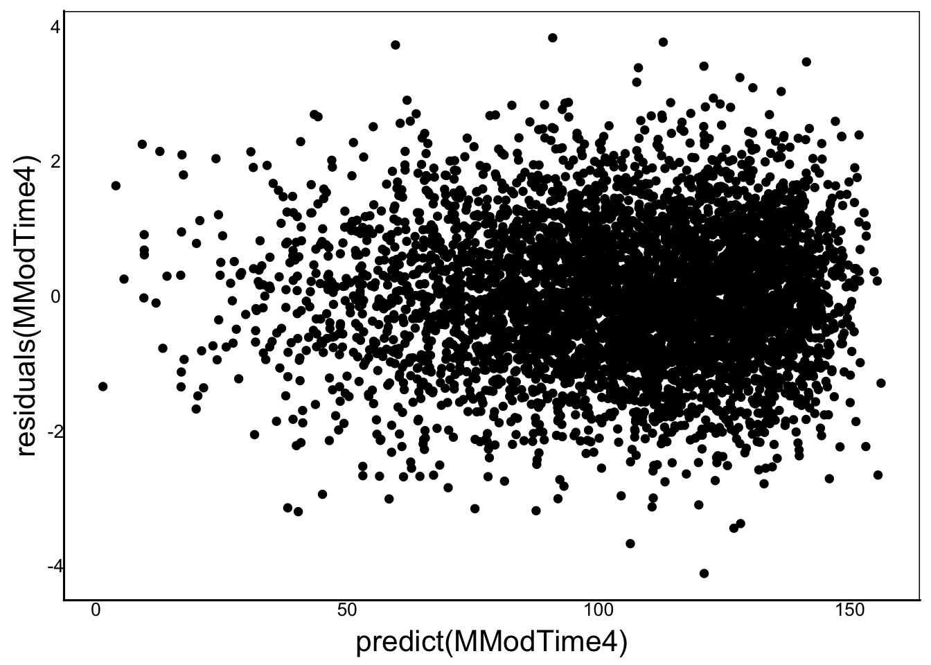

ggplot() + 
  stat_qq(aes(sample=residuals(MModTime4))) + 
  stat_qq_line(aes(sample=residuals(MModTime4)))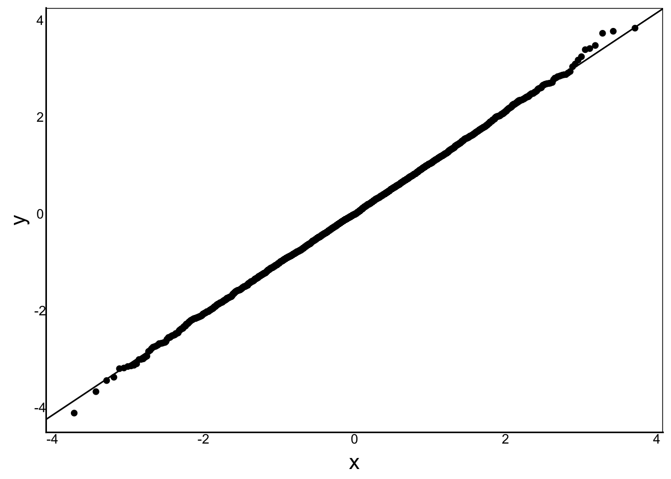

Generalized LME

Linear Mixed Effects Models (LMEs) with lmer are the mixed-model equivalent of linear models with lm.

Just as we could use glm with the family= parameter to fit generlized linear models, we can use the family= parameter in glmer to fit Generalized Linear Mixed Effects Models.

You should be comfortable with the difference between glm and lm, so you shouldn’t have much problem moving from lmer to glmer. We’ll do one quick example: imagine we are looking at counts of immune cells rather than IgG concentration. Let’s set this up by creating a Cells column that is a function of our IgG levels. We’ll also filter for only females to make the model a bit easier:

CellDat<-ImmuneDat %>% 
  filter(Sex=="F") %>%
  mutate(Cells=round(IgG^1.2,0))

Now run the Generalized Linear Mixed Effects Model. Note that we will change response variable to Cells instead of IgG, from the CellDat data instead of ImmuneDat. Additionally, we have added a distribution family for the residuals to make this a generalized model, just as you might do when converting from lm to glm.

One more thing: we add nAGQ=0 to the model to increase speed in the model parameter estimation, which should also help us avoid convergence errors. After entering the model below, note how much longer it takes to run this model compared to lmer, even though we are estimating a much simpler model from a data set half the size (i.e., females only).

GMModTime<-glmer(Cells ~ Time + (Time|FamID) + 
                   (Time|IndID), data=CellDat,
                family=poisson, nAGQ=0)
summary(GMModTime)

Generalized linear mixed model fit by maximum likelihood (Adaptive
  Gauss-Hermite Quadrature, nAGQ = 0) [glmerMod]
 Family: poisson  ( log )
Formula: Cells ~ Time + (Time | FamID) + (Time | IndID)
   Data: CellDat

      AIC       BIC    logLik -2*log(L)  df.resid 
  19503.2   19549.6   -9743.6   19487.2      2422 

Scaled residuals: 
    Min      1Q  Median      3Q     Max 
-3.9881 -0.2399  0.0486  0.3087  1.6476 

Random effects:
 Groups Name        Variance  Std.Dev. Corr  
 IndID  (Intercept) 0.0002517 0.01586        
        Time        0.0001810 0.01345  -0.65 
 FamID  (Intercept) 0.0010976 0.03313        
        Time        0.0001445 0.01202  0.33  
Number of obs: 2430, groups:  IndID, 135; FamID, 8

Fixed effects:
             Estimate Std. Error z value Pr(>|z|)    
(Intercept)  5.955729   0.011995  496.53   <2e-16 ***
Time        -0.044323   0.004415  -10.04   <2e-16 ***
---
Signif. codes:  0 '***' 0.001 '**' 0.01 '*' 0.05 '.' 0.1 ' ' 1

Correlation of Fixed Effects:
     (Intr)
Time 0.286