library(ggplot2) # plotting libraryWarning: package 'ggplot2' was built under R version 4.5.2library(dplyr) # data management
source("http://bit.ly/theme_pub") # Set custom plotting theme
theme_set(theme_pub())Linear models are run in R using the lm() function, as we saw detailed in the Linear Models Tutorial. In that tutorial, we also saw a wide range of ‘classical’ statistical models that differ only in the type of predictor variables (e.g. ANOVA for categorical and regression for continuous).
We also learned how to inspect our residuals to make sure that they don’t violate model assumptions. One of the most important is that the error term follows a normal distribution with a mean of zero.
Generalized Linear Models are very similar in the way they are programmed, except that they use the glm() function in R, rather than lm(), and they can be used when our residuals DO NOT follow a normal distribution. If you understand how lm works, then glm will be very easy to understand. If you are still struggling with lm then it’s a good idea to go back and review/practice before continuing.
All Linear Models are Generalized Linear Models with a normal error distribution, but additionally we can use other error distributions like the Poisson, and the binomial. We specify the error distribution with the family= parameter in glm(). If you click on the family link in the glm help, you will see that each error distribution includes a link= parameter. For example, gaussian(link="identity"), binomial(link="logit"), and poisson(link="log"). A link function transforms the linear model to the scale of the error term. We’ll show how this works for Logistic Regression (binomial response variable) and Poisson Regression (log-normal or count response variable). Note that the Gaussian uses the identity link, meaning that the model is not transformed.
Load libraries and custom plotting theme
library(ggplot2) # plotting libraryWarning: package 'ggplot2' was built under R version 4.5.2library(dplyr) # data management
source("http://bit.ly/theme_pub") # Set custom plotting theme
theme_set(theme_pub())Let’s start with a typical linear model by generating pretend data:
N<-1000
X1<-rnorm(N, sd=3)
X2<-sample(c("Control","Treat1"), N, replace=T)
tDat<-data.frame(Pred1=X1, Pred2=X2) %>%
  mutate(Pred2dev=recode(Pred2, "Control"=0, "Treat1"=4)) %>%
  mutate(Resp= -1 + 0.3*Pred1 + Pred2dev + rnorm(N, sd=2))
This is similar to the models we set up in the Linear Models Tutorial, where we have a sample size of N = 1000, we have a continuous predictor and we have a categorical predictor. Our response variable is a function of the predictors with a slope of \(0.3 \times X_1\) and a random normal error. We add the strings for the treatment category so that we can run the linear model.
Mod<-lm(Resp~Pred1 + Pred2, data=tDat)
summary(Mod)
Call:
lm(formula = Resp ~ Pred1 + Pred2, data = tDat)

Residuals:
    Min      1Q  Median      3Q     Max
-6.1794 -1.3564 -0.0736  1.3306  6.9179

Coefficients:
            Estimate Std. Error t value Pr(>|t|)
(Intercept) -0.96720    0.09024  -10.72   <2e-16 ***
Pred1        0.28799    0.02186   13.18   <2e-16 ***
Pred2Treat1  4.00806    0.12718   31.52   <2e-16 ***
---
Signif. codes:  0 '***' 0.001 '**' 0.01 '*' 0.05 '.' 0.1 ' ' 1

Residual standard error: 2.009 on 997 degrees of freedom
Multiple R-squared:  0.532, Adjusted R-squared:  0.531
F-statistic: 566.6 on 2 and 997 DF,  p-value: < 2.2e-16
Recall that the model is:
\[ Y = \beta_0 + \beta_1*X_1 + \beta_2X_2 + \epsilon \]
where \(Y\) is a vector (e.g. column in a data frame) containing the response values for each individual, \(\Beta_0\) is the intercept of the model, \(\beta_1\) is the slope of the predictor \(X_1\), which is also a vector containing values for the first predictor. \(\beta_2\) is likewise the slope for the vector of predictor \(X_2\) and \(\epsilon\) is the residual error term.
The key assumption that distinguishes lm from glm is that our residual error is normally distributed:
ggplot() +
  geom_histogram(aes(x=residuals(Mod)))
`stat_bin()` using `bins = 30`. Pick better value `binwidth`.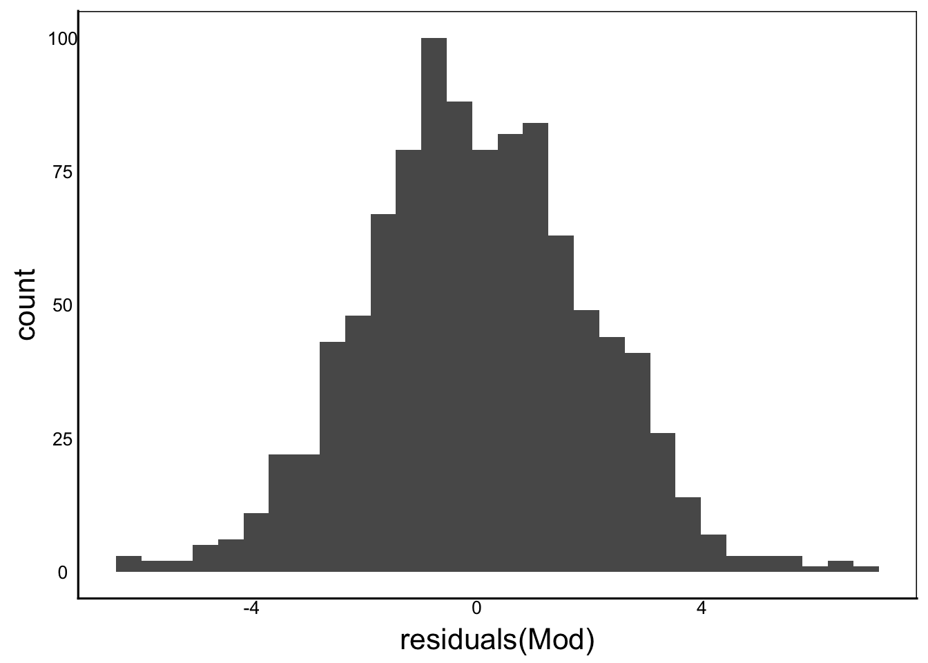
We can fit the same model using GLM. Compare this code to the lm model, above:
GLMod<-glm(Resp~Pred1 + Pred2, family=gaussian, data=tDat)Note the addition of the family= parameter. Here we use Gaussian, which is also the default – so technically we don’t need to specify it for this model. However, we include it here for now and then change the family to fit different error distributions.
Now compare the output:
summary(GLMod)
Call:
glm(formula = Resp ~ Pred1 + Pred2, family = gaussian, data = tDat)

Coefficients:
            Estimate Std. Error t value Pr(>|t|)
(Intercept) -0.96720    0.09024  -10.72   <2e-16 ***
Pred1        0.28799    0.02186   13.18   <2e-16 ***
Pred2Treat1  4.00806    0.12718   31.52   <2e-16 ***
---
Signif. codes:  0 '***' 0.001 '**' 0.01 '*' 0.05 '.' 0.1 ' ' 1

(Dispersion parameter for gaussian family taken to be 4.035953)

    Null deviance: 8597.1  on 999  degrees of freedom
Residual deviance: 4023.8  on 997  degrees of freedom
AIC: 4238.1

Number of Fisher Scoring iterations: 2
It should be very similar, but you’ll notice that there is no p-value for the overall model. But, there is an AIC that we can use for model selection, or we can do the likelihood ratio test. You can review these in the Model Selection Tutorial if you need a refresher.
library(lmtest)Loading required package: zoo
Attaching package: 'zoo'The following objects are masked from 'package:base':
as.Date, as.Date.numericGLMod2<-glm(Resp~Pred1, data=tDat)
lrtest(GLMod2,GLMod)Likelihood ratio test
Model 1: Resp ~ Pred1
Model 2: Resp ~ Pred1 + Pred2
#Df LogLik Df Chisq Pr(>Chisq)
1 3 -2460.7
2 4 -2115.1 1 691.23 < 2.2e-16 ***
---
Signif. codes: 0 '***' 0.001 '**' 0.01 '*' 0.05 '.' 0.1 ' ' 1Now what if our residuals are not from a random normal distribution? First, make sure you review the Distributions Tutorial.
A Logistic Regression is similar to a linear regression in lm() except that the response variable is binary rather than continuous. This means that values of the response variable must be either 0 or 1. This is also known as a Bernoulli variable. Going back to our Distributions Tutorial you may recall that we can sample from a random binomial distribution with the rbinom distribution. In this case, the ‘size’ parameter is just 1 because each response observation is a 0 or 1. But to generate a statistical model, we have to define the probability of 0 and 1. We also have to make sure that the probabilities add up to 1. In a logistic regression this is done with a transformation of the linear model (Y) to a probability (P). This is called Link function:
\[P = \frac{1}{1+e^{-Y}} \]
Or more specifically: \[ P = \frac{1}{1+e^{-(\beta_0 + \beta_1*X_1 + \beta_2X_2)}} \]
Note that the residual error is not part of the link function
Logit<-1/(1+exp(-(-1 + 0.3*tDat$Pred1 + tDat$Pred2dev)))
ggplot()+
  geom_point(aes(x=tDat$Resp,y=Logit))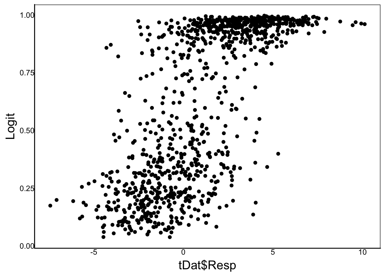
Notice how the y-axis runs from 0 to 1, which we can think of as a probability of observing 1 in the dataset. Now we can input that probability
tDat<-tDat %>%
  mutate(LResp=rbinom(n=N, size=1, prob=Logit))
To run the glm model, we have to specify that this is a logistic model, rather than Gaussian.
LMod<-glm(LResp ~ Pred1 + Pred2, family=binomial, data=tDat)
summary(LMod)
Call:
glm(formula = LResp ~ Pred1 + Pred2, family = binomial, data = tDat)

Coefficients:
            Estimate Std. Error z value Pr(>|z|)
(Intercept) -1.01935    0.11007  -9.261   <2e-16 ***
Pred1        0.31484    0.03592   8.765   <2e-16 ***
Pred2Treat1  4.15679    0.24767  16.784   <2e-16 ***
---
Signif. codes:  0 '***' 0.001 '**' 0.01 '*' 0.05 '.' 0.1 ' ' 1

(Dispersion parameter for binomial family taken to be 1)

    Null deviance: 1326.2  on 999  degrees of freedom
Residual deviance:  747.5  on 997  degrees of freedom
AIC: 753.5

Number of Fisher Scoring iterations: 5
Note how the estimates are very similar to the gaussian model BUT REMEMBER that to generate our predictions we have to transform our linear model using the equation above. You can see the difference by re-running the model with lm (without the family parameter) and seeing how the Estimate values differ.
As with the gaussian distribution, we can use LRT to determine the significance of specific terms or models, or AIC for more general model selection.
A logistic regression is a glm with a binomial error distribution and a response variable that is coded as binary (0 or 1). But what if our response variable is a proportion or count data? For example, what if we were studying whether a mother’s exposure to a particular environmental chemical increased their offsprings probability of developing cancer? Whether a particular child develops cancer is a binary even (0 or 1) but each mother has a different number of children (say, between 1 and 7).
In cases like these, we can specify two columns as a single response variable in our glm – one for the number of children with cancer (cancer), and another for the number of children without cancer (nocancer). Our model would look like this:
glm(cbind(cancer,nocancer) ~ environment, family=binomial)This model won’t run, because we haven’t generated the data yet. But note how our response variable uses the cbind command, to link to columns together as a single response variable.
Alternatively, we might have the data encoded as a single column for the proportion of children with cancer (pcancer) and the total number of children (nchild) for each maternal family. In that case, we can use the proportion as the response with the number of children as a weight. We use weights because 5 of 10 is a more reliable estimate of 0.5 than 1 of 2. If each maternal family had the same number of offspring sampled, or if we didn’t know the total number of children in each family, then we wouldn’t need to use the weight parameter because all would be weighted equally.
glm(pcancer ~ environment, weights=nchild, family=binomial)Again, the above code won’t run, but it shows the general form of a model with a proportion as the response and a data column for weights.
As discussed in previous chapters, Poisson variables are common for count data (e.g. N offspring) but also can apply to log-normally distributed data with continuous measurements (e.g. biomass).
If we look at rpois() to sample from a Poisson distribution, we can see the term lambda, which is the mean of the poisson distribution. In a Poisson distribution, the variance (e.g. residual error) scales with the mean. Specifically, the prediction is on the natural-log scale:
\[ N = e^{Y}\]
Or the more detailed version:
\[ N = e^{\beta_0 + \beta_1*X_1 + \beta_2X_2}\]
Similar to the logistic regression, we transform the model using the link equation.
Log<-exp(-1 + 0.3*tDat$Pred1 + tDat$Pred2dev)
tDat<-tDat %>%
  mutate(PResp=rpois(N, lambda=Log))
And we can plot our Gaussian response (Resp) against our Poisson response (PResp) to better understand the relationship
ggplot(aes(x=Resp,y=PResp,colour=Pred2),data=tDat) +
  geom_point()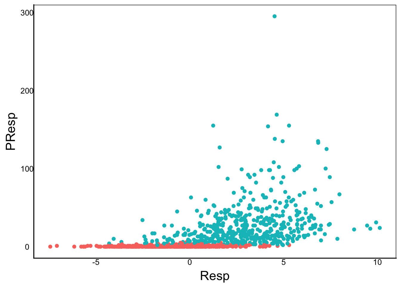
Now run the model and compare the output.
PMod<-glm(PResp ~ Pred1 + Pred2,
          family=poisson(link="log"), data=tDat)
summary(PMod)
Call:
glm(formula = PResp ~ Pred1 + Pred2, family = poisson(link = "log"),
    data = tDat)

Coefficients:
             Estimate Std. Error z value Pr(>|z|)
(Intercept) -0.912726   0.058244  -15.67   <2e-16 ***
Pred1        0.302779   0.002955  102.46   <2e-16 ***
Pred2Treat1  3.906880   0.058341   66.97   <2e-16 ***
---
Signif. codes:  0 '***' 0.001 '**' 0.01 '*' 0.05 '.' 0.1 ' ' 1

(Dispersion parameter for poisson family taken to be 1)

    Null deviance: 28927.61  on 999  degrees of freedom
Residual deviance:   907.75  on 997  degrees of freedom
AIC: 3756

Number of Fisher Scoring iterations: 5?family provides a list of families that you can use with glm and related models. Of particular note are the quasi, quasibinomial, and quasipoisson families. These are similar to the gaussian, binomial, and poisson, respectively, except that they allow for overdispersion of the error distribution.
Sometimes the link function is obvious given the data. For example, a response variable with 1 and 0 would be a binomial function in our example above. But sometimes it’s not so easy. For example, other families not covered here can give the same response data type. In these cases, we can use information criteria to test the fit of different models. We can see an example of this for our poisson model:
GausMod<-glm(PResp ~ Pred1 + Pred2, family=gaussian, data=tDat)
PoisMod<-glm(PResp ~ Pred1 + Pred2, family=poisson, data=tDat)
AIC(GausMod)
[1] 8472.139AIC(PoisMod)[1] 3756.039We can see the model with the poisson link fits much better than the model with the Gaussian link.
Question: Why can’t we use a likelihood ratio test?
Answer: We are changing the error distribution only. Since the models are not ‘nested’, we have 0 degrees of freedom to do a LRT.
We can use the same QA/QC protocols for glm that we use for lm (see the Linear Models chapter for details).
One quick example:
library(ggfortify)
ggplot() +
  geom_histogram(aes(residuals(PMod)))
`stat_bin()` using `bins = 30`. Pick better value `binwidth`.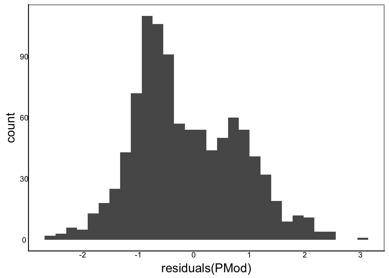
Note the apparent structure when residuals < 0 in the residuals plot.
autoplot(PMod, which=1, data=tDat, colour = 'Pred2')Warning: `fortify(<lm>)` was deprecated in ggplot2 4.0.0.
ℹ Please use `broom::augment(<lm>)` instead.
ℹ The deprecated feature was likely used in the ggfortify package.
Please report the issue at <https://github.com/sinhrks/ggfortify/issues>.Warning: `aes_string()` was deprecated in ggplot2 3.0.0.
ℹ Please use tidy evaluation idioms with `aes()`.
ℹ See also `vignette("ggplot2-in-packages")` for more information.
ℹ The deprecated feature was likely used in the ggfortify package.
Please report the issue at <https://github.com/sinhrks/ggfortify/issues>.Warning: Using `size` aesthetic for lines was deprecated in ggplot2 3.4.0.
ℹ Please use `linewidth` instead.
ℹ The deprecated feature was likely used in the ggfortify package.
Please report the issue at <https://github.com/sinhrks/ggfortify/issues>.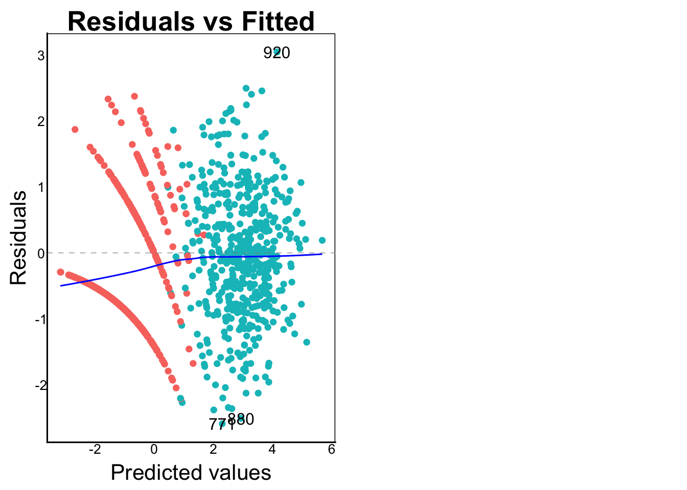
autoplot(PMod, which=2, data=tDat, colour = 'Pred2')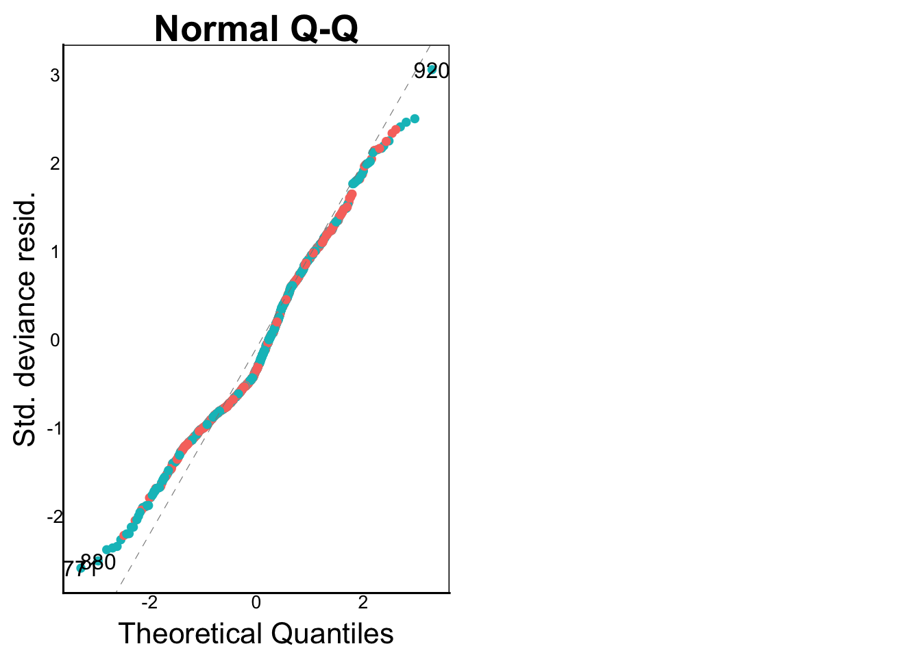
autoplot(PMod, which=3, data=tDat, colour = 'Pred2')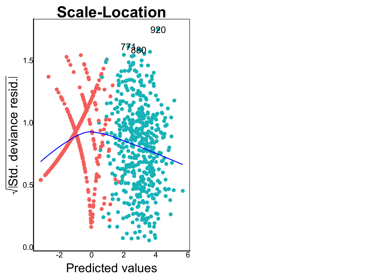
autoplot(PMod, which=4, data=tDat, colour = 'Pred2')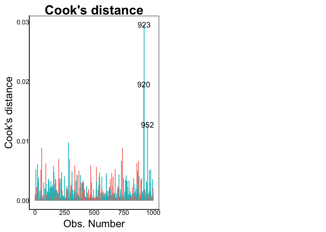
Again, note the apparent structure when Predicted values < 0. This is just an artifact of the Poisson sampling with means < 1, since we can’t have any values between 0 and 1. What we really have is a mixed dataset with Logistic data for small predicted values and Poisson data for larger values.
Question: Try re-running PMod with a logistic and then a gaussian family and compare the residuals to this. Which residuals look best?